Data Transformation in Machine Learning
Data transformation is the backbone of every ML pipeline -- the stage where raw, messy, heterogeneous data gets reshaped into clean, structured, model-ready features. Without it, even the most sophisticated model architecture is eating garbage for breakfast.
In the broadest sense, data transformation encompasses every operation that changes the structure, format, or values of your data between ingestion and model consumption. That includes joins across data sources, aggregations that create summary statistics, type conversions, pivoting and unpivoting, log and power transformations, time-series resampling, encoding categorical variables, and constructing feature crosses. It is the single most time-consuming phase of any ML project -- estimates consistently place it at 60-80% of total engineering effort.
The tools landscape spans from single-machine libraries like Pandas and Polars, through SQL-based transformation frameworks like dbt, all the way to distributed engines like Apache Spark and Apache Beam. Choosing the right tool at the right scale is itself a design decision that separates teams who ship from teams who struggle. From Flipkart's 35+ PB data platform running 25,000 compute pipelines to a bootstrapped startup in Bengaluru running dbt on Snowflake, data transformation is where the engineering rubber meets the ML road.
This guide covers the theory, architecture, implementation patterns, failure modes, and production tradeoffs you need to design robust data transformation stages in real-world ML systems.
Concept Snapshot
- What It Is
- The process of converting raw data into a structured, clean, feature-rich format suitable for machine learning model training and inference through operations like joins, aggregations, encoding, normalization, and reshaping.
- Category
- Data Processing
- Complexity
- Intermediate
- Inputs / Outputs
- Inputs: raw data from batch or streaming sources (CSVs, databases, event streams, APIs). Outputs: cleaned, joined, aggregated, and feature-engineered datasets ready for model training or serving.
- System Placement
- Sits after data ingestion/extraction and data cleaning, and before feature extraction, feature stores, or direct model training in the ML pipeline.
- Also Known As
- data wrangling, data munging, data preprocessing, ETL transformation layer, feature transformation, data reshaping
- Typical Users
- Data Engineers, ML Engineers, Data Scientists, Analytics Engineers, Platform Engineers
- Prerequisites
- SQL fundamentals, DataFrame operations (Pandas/Spark), Basic statistics (mean, median, variance), Data modeling concepts (star schema, normalization)
- Key Terms
- ETLELTjoinaggregationpivotunpivotfeature crosslog transformationone-hot encodingresamplingidempotentlineage
Why This Concept Exists
Raw Data Is Never Model-Ready
Here is an uncomfortable truth: real-world data is a mess. It arrives in different formats (JSON, CSV, Parquet, Avro), from different systems (MySQL, Kafka, S3, REST APIs), with different schemas, different time zones, different levels of completeness, and different definitions of what "null" means. A transaction table in one system records amounts in paise (1/100th of a rupee), while another uses whole rupees. A user table stores dates as Unix timestamps; another uses ISO 8601 strings. An event stream delivers nested JSON; a batch export delivers flat CSV.
No ML model can consume this directly. You need a systematic process to harmonize, reshape, and enrich this data before it becomes useful. That process is data transformation.
The Historical Arc: ETL to ELT to ML-Aware Pipelines
Data transformation has a long history in data engineering. The classic ETL (Extract-Transform-Load) pattern, dating back to the data warehousing era of the 1990s, performed transformations on a dedicated ETL server before loading into the warehouse. Tools like Informatica and Talend dominated this space.
The rise of cloud data warehouses (BigQuery, Snowflake, Redshift) inverted this pattern into ELT (Extract-Load-Transform). Raw data is loaded first, and transformations happen inside the warehouse using SQL -- leveraging the warehouse's own compute engine. dbt (data build tool) emerged as the de facto standard for managing these SQL-based transformations with version control, testing, and dependency management.
But ML pipelines introduced a third evolution. ML transformations often need to be applied identically at training time and serving time -- what Google calls "training-serving skew" prevention. This led to tools like TensorFlow Transform (tf.Transform) that define transformations as code that can execute both in batch during training and in real-time during inference. The transformation is no longer just a data engineering concern; it is a model correctness concern.
Key Insight: The shift from ETL to ELT to ML-aware transformation pipelines reflects a fundamental change: transformations are no longer just about getting data into a warehouse. They are about producing features that must be consistent across training, validation, and production serving.
Why ML Makes This Harder
Traditional BI transformations produce dashboards and reports -- if a transformation has a bug, someone notices a wrong number on a chart. ML transformations produce features that feed statistical models -- if a transformation has a bug, the model silently learns the wrong patterns. There is no dashboard to eyeball. The feedback loop is longer, the failure mode is subtler, and the cost of getting it wrong is higher.
This is why data transformation in ML systems demands more rigor than traditional data engineering: schema enforcement, data validation checks at every stage, idempotent pipelines, and reproducible transformations that can be audited months later.
Core Intuition & Mental Model
The Assembly Line Analogy
Think of data transformation as an assembly line in a factory. Raw materials (data) arrive at the loading dock in different shapes and sizes -- some in crates, some loose, some damaged. The assembly line's job is to inspect each piece, reshape it to standard dimensions, combine components that belong together (joins), stamp quality marks (validation), and package the final product (feature vectors) for the next station (the model).
Just like a real assembly line, the order of operations matters. You would not paint a car before welding the body panels. Similarly, you would not one-hot encode a categorical column before cleaning its inconsistent values ("Mumbai", "mumbai", "MUMBAI" should be one category, not three).
Three Mental Models for Transformation
Mental Model 1: Shape-Changing. Many transformations are about changing the shape of your data. A pivot turns rows into columns. An aggregation collapses many rows into one. A join widens a table by adding columns from another table. An explode takes one row with an array and turns it into many rows. Think of your data as clay -- transformation is the sculpting.
Mental Model 2: Information Enrichment. Some transformations do not change the data itself but add derived information. A feature cross multiplies two columns together to capture their interaction. A rolling window average adds temporal context. A log transformation rescales values to make patterns visible. You are not moving data around; you are creating new signals from existing ones.
Mental Model 3: Consistency Enforcement. The third class of transformations ensures that data conforms to expectations. Type casting, timezone normalization, unit conversion, deduplication -- these transformations do not add information; they remove ambiguity. They ensure that when your model sees "price = 100," it always means 100 INR, not sometimes 100 paise.
The Core Promise: Data transformation takes heterogeneous, messy inputs and produces homogeneous, reliable outputs that a statistical model can learn from. Without it, your model is learning from noise.
Technical Foundations
Formalizing Transformation Operations
A data transformation pipeline can be formalized as a directed acyclic graph (DAG) of operators. Let be the input dataset and be the output. A pipeline is a composition of transformation functions:
where each is a transformation operator over the space of tabular datasets .
Common Operator Classes
1. Projection (Column Selection): where retains only columns from .
2. Aggregation: where is the grouping key and is an aggregate function (sum, mean, count, etc.).
3. Join: Combines rows from and where key columns match. The choice of join type (inner, left, outer, cross) determines how unmatched rows are handled.
4. Log Transformation: where is a small constant to handle zeros. This is ubiquitous for right-skewed distributions like transaction amounts, where a few high-value orders (say, a Diwali sale bulk purchase on Flipkart) dominate the raw distribution.
5. Feature Cross:
or more generally, for arbitrary interaction functions. Feature crosses capture non-linear interactions that linear models cannot learn on their own. For example, crossing city and cuisine_type in a Zomato recommendation model captures that biryani is popular in Hyderabad but less so in Chennai.
6. Time-Series Resampling: Given a time series with irregular timestamps, resampling produces a regular series where for a chosen frequency . The resampled value is computed via interpolation, forward-fill, or aggregation over the interval .
Idempotency Property
A critical property for production transformation pipelines is idempotency: applying the same transformation twice yields the same result as applying it once.
This ensures that pipeline retries (inevitable in production) do not corrupt data. Achieving idempotency typically requires using MERGE / UPSERT semantics rather than INSERT for write operations, and designing transformations that are deterministic given the same input partition.
Computational Complexity
The cost of transformation depends heavily on the operator:
| Operation | Time Complexity | Bottleneck |
|---|---|---|
| Filter / Map | CPU | |
| Sort | Memory | |
| Hash Join | Memory for hash table | |
| Sort-Merge Join | I/O | |
| Group-By Aggregation | amortized | Memory for hash map |
| Window Function | CPU, where is window size |
At scale (billions of rows), the constants matter enormously -- this is why distributed engines like Spark partition data across nodes and process partitions in parallel.
Internal Architecture
A data transformation system in an ML pipeline consists of several interconnected layers: a source connector layer that reads from heterogeneous data sources, a computation engine that executes transformation logic, a metadata and lineage layer that tracks what happened to each record, a quality gate that validates outputs, and a sink layer that writes results to downstream storage.
The architecture differs significantly depending on whether you are doing batch or streaming transformations, and whether you are on a single machine or a distributed cluster. But the logical flow is consistent across all implementations.
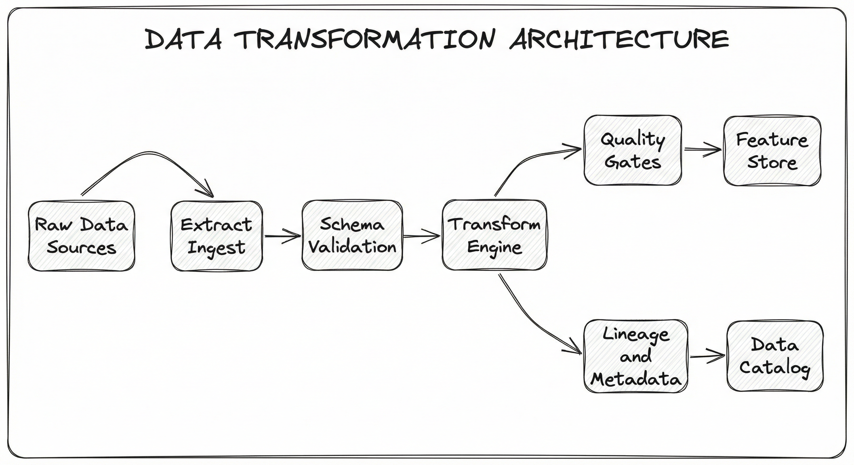
In a modern ML pipeline, the transform engine is the heaviest component. It handles joins across multiple data sources (e.g., joining user profiles from a PostgreSQL database with clickstream events from Kafka), applies aggregations (e.g., computing 7-day rolling averages of user engagement), performs encoding (e.g., one-hot encoding of categorical features), and generates derived features (e.g., feature crosses between geographic region and product category).
The quality gates are non-negotiable in production. They run statistical checks on transformation outputs -- verifying that column distributions haven't shifted unexpectedly, that null rates are within bounds, and that row counts match expectations. Without these gates, a subtle upstream schema change can silently corrupt your entire feature set.
Key Components
Source Connectors
Read data from heterogeneous sources -- relational databases (MySQL, PostgreSQL), object storage (S3, GCS), message queues (Kafka, Pub/Sub), APIs, and file formats (CSV, Parquet, Avro, JSON). Handle schema inference, partitioning, and incremental reads.
Schema Registry / Validator
Enforces expected schemas on incoming data before transformation begins. Catches type mismatches, missing columns, and unexpected nulls early -- before they propagate through the pipeline and corrupt downstream features.
Transform Engine
The core computation layer. Executes transformation logic -- joins, aggregations, window functions, encoding, feature crosses, and custom UDFs. Can be a single-machine engine (Pandas, Polars, DuckDB) or a distributed engine (Spark, Beam, Flink). This is where 90% of the compute budget goes.
Orchestrator
Manages the DAG of transformation steps, handles scheduling, retries, and dependency resolution. Tools include Apache Airflow, Dagster, Prefect, and Spotify's Flyte. Ensures transformations run in the correct order and handles failures gracefully.
Quality Gates
Runs post-transformation validation checks: statistical distribution tests, null rate assertions, row count expectations, referential integrity checks. Tools like Great Expectations and dbt tests provide declarative quality assertion frameworks.
Lineage Tracker
Records the provenance of every output column -- which source columns, transformations, and code versions produced it. Critical for debugging, auditing, and regulatory compliance. Tools like Apache Atlas, DataHub, and OpenLineage provide lineage graph capabilities.
Sink / Writer
Writes transformed data to downstream storage -- feature stores (Feast, Tecton), data warehouses (BigQuery, Snowflake, Redshift), or direct model input formats (TFRecord, Parquet). Handles partitioning, compaction, and write optimization.
Data Flow
Batch Path: Orchestrator triggers extraction from source systems -> raw data lands in a staging area (e.g., S3 raw zone) -> schema validator checks incoming data against expected contracts -> transform engine reads validated data, applies the transformation DAG (joins, aggregations, encoding, feature generation) -> quality gates verify output statistics against expectations -> validated features are written to the feature store or model training dataset -> lineage metadata is recorded in the data catalog.
Streaming Path: Events arrive continuously via Kafka or Pub/Sub -> a stream processor (Flink, Spark Structured Streaming, Beam) applies windowed transformations in near-real-time -> results are written to a low-latency store (Redis, DynamoDB) for online serving -> the same transformation logic (ideally from a shared codebase) runs in batch for training data generation, ensuring training-serving consistency.
Hybrid Path (Most Common in Production): Batch transformations run on a schedule (hourly, daily) to produce training datasets and backfill features. Streaming transformations run continuously for online features that require freshness (e.g., a user's last-5-minutes activity count). Both paths write to a unified feature store that serves both training and inference.
A directed flow from 'Raw Data Sources' through 'Extract/Ingest', 'Schema Validation', 'Transform Engine', and 'Quality Gates' to 'Feature Store / Model Input'. A parallel branch from 'Transform Engine' flows to 'Lineage & Metadata' and then to 'Data Catalog'. The Transform Engine is the central, heaviest component.
How to Implement
Choosing Your Transformation Engine
The choice of transformation engine depends on three factors: data volume, latency requirements, and team expertise.
For datasets that fit in memory (up to ~50 GB on a modern machine), single-machine tools are often the best choice. Pandas is the incumbent -- ubiquitous, well-documented, and supported by virtually every ML library. Polars is the modern challenger -- written in Rust, it delivers 5-30x performance improvements over Pandas on large datasets through lazy evaluation, multi-threaded execution, and columnar memory layout. DuckDB offers SQL-based transformation on local files with surprising performance.
For datasets that exceed single-machine capacity (100 GB to petabytes), distributed engines are necessary. Apache Spark (via PySpark) is the workhorse -- used by Uber for 2M+ daily Spark applications, by Netflix for 500B+ daily events, and by Flipkart across their 800+ node Hadoop cluster. Apache Beam provides a unified API that runs on multiple backends (Dataflow, Flink, Spark), and is used by Spotify across their 20,000+ data pipelines.
For SQL-first transformation workflows, dbt has become the standard. It lets analytics engineers write modular, testable SQL transformations with dependency management, documentation, and data quality tests built in. dbt runs inside your data warehouse (BigQuery, Snowflake, Redshift, Databricks), leveraging the warehouse's own compute engine.
For ML-specific transformations that must be consistent between training and serving, TensorFlow Transform (tf.Transform) and Spark MLlib Pipelines provide transformation definitions that can be exported and applied at inference time.
Cost Context: Running a 10-node Spark cluster on AWS EMR (m5.xlarge instances) costs approximately 7/day (~INR 590/day) or ~2-5 per transformation run depending on warehouse size, roughly $60-150/month (~INR 5,000-12,600/month) for moderate workloads.
from pyspark.sql import SparkSession
from pyspark.sql import functions as F
from pyspark.sql.window import Window

spark = SparkSession.builder \
    .appName("MLFeatureTransformation") \
    .config("spark.sql.shuffle.partitions", 200) \
    .getOrCreate()

# Read from multiple sources
orders = spark.read.parquet("s3://data-lake/raw/orders/")
users = spark.read.parquet("s3://data-lake/raw/users/")
products = spark.read.parquet("s3://data-lake/raw/products/")

# Join orders with user and product dimensions
enriched = orders \
    .join(users, orders.user_id == users.id, "left") \
    .join(products, orders.product_id == products.id, "left")

# Aggregation: user-level features
user_features = enriched.groupBy("user_id").agg(
    F.count("order_id").alias("total_orders"),
    F.sum("amount_inr").alias("lifetime_value_inr"),
    F.avg("amount_inr").alias("avg_order_value_inr"),
    F.countDistinct("category").alias("unique_categories"),
    F.datediff(F.max("order_date"), F.min("order_date")).alias("tenure_days")
)

# Window function: rolling 30-day order count
window_30d = Window.partitionBy("user_id") \
    .orderBy(F.col("order_date").cast("long")) \
    .rangeBetween(-30 * 86400, 0)

orders_with_rolling = enriched.withColumn(
    "orders_last_30d",
    F.count("order_id").over(window_30d)
)

# Log transformation for skewed monetary features
user_features = user_features.withColumn(
    "log_lifetime_value",
    F.log1p(F.col("lifetime_value_inr"))
)

# Feature cross: city x category interaction
enriched = enriched.withColumn(
    "city_category_cross",
    F.concat_ws("_", F.col("city"), F.col("category"))
)

# Write to feature store
user_features.write \
    .mode("overwrite") \
    .partitionBy("signup_month") \
    .parquet("s3://data-lake/features/user_features/")
This PySpark example demonstrates a typical ML feature engineering pipeline: reading from multiple data sources, performing joins to create an enriched dataset, computing user-level aggregations for features like lifetime value and order frequency, applying window functions for temporal features (rolling 30-day counts), using log transformations to handle skewed distributions, and constructing feature crosses that capture interaction effects. The output is partitioned and written to a feature storage layer. This pattern is used at companies like Flipkart and Swiggy to build user-level features from transactional data.
-- models/features/user_order_features.sql
-- dbt model: Computes user-level order features for ML

{{ config(
    materialized='incremental',
    unique_key='user_id',
    partition_by={'field': 'computed_at', 'data_type': 'date'},
    tags=['ml-features', 'daily']
) }}

WITH order_history AS (
    SELECT
        user_id,
        order_id,
        amount_inr,
        order_date,
        category,
        city
    FROM {{ ref('stg_orders') }}
    {% if is_incremental() %}
    WHERE order_date > (SELECT MAX(order_date) FROM {{ this }})
    {% endif %}
),

user_aggregates AS (
    SELECT
        user_id,
        COUNT(DISTINCT order_id) AS total_orders,
        SUM(amount_inr) AS lifetime_value_inr,
        AVG(amount_inr) AS avg_order_value_inr,
        COUNT(DISTINCT category) AS unique_categories,
        DATE_DIFF(MAX(order_date), MIN(order_date), DAY) AS tenure_days,
        LN(SUM(amount_inr) + 1) AS log_lifetime_value,
        CURRENT_DATE() AS computed_at
    FROM order_history
    GROUP BY user_id
)

SELECT * FROM user_aggregates

-- schema.yml (tests and documentation)
-- version: 2
-- models:
--   - name: user_order_features
--     description: "User-level order features for churn prediction model"
--     columns:
--       - name: user_id
--         tests:
--           - unique
--           - not_null
--       - name: lifetime_value_inr
--         tests:
--           - not_null
--           - dbt_utils.accepted_range:
--               min_value: 0
This dbt model shows SQL-based transformation with production-grade features: incremental materialization (only processing new data), partitioning for efficient queries, and embedded data quality tests. The model computes the same user-level features as the Spark example but using pure SQL inside the data warehouse. dbt's ref() function handles dependency management, and the schema tests ensure data quality on every run. This pattern is increasingly popular at companies using dbt with Snowflake or BigQuery for ML feature pipelines.
import polars as pl

# Read data with lazy evaluation
orders = pl.scan_parquet("data/orders/*.parquet")
users = pl.scan_parquet("data/users/*.parquet")

# Define transformation pipeline lazily
features = (
    orders
    .join(users, on="user_id", how="left")
    # Time-series resampling: aggregate to daily level
    .with_columns(
        pl.col("order_timestamp").dt.date().alias("order_date")
    )
    .group_by(["user_id", "order_date"])
    .agg([
        pl.col("amount_inr").sum().alias("daily_spend_inr"),
        pl.col("order_id").count().alias("daily_order_count"),
        pl.col("category").n_unique().alias("daily_unique_categories"),
    ])
    # Log transformation
    .with_columns(
        pl.col("daily_spend_inr").log1p().alias("log_daily_spend")
    )
    # Pivot: category spend as columns
    .collect()  # Materialize before pivot
)

# Pivot operation: create category-level spend columns
category_pivot = (
    orders
    .collect()
    .pivot(
        on="category",
        index="user_id",
        values="amount_inr",
        aggregate_function="sum"
    )
    .fill_null(0)
)

# Feature cross using expressions
features = features.with_columns(
    (pl.col("daily_order_count") * pl.col("daily_unique_categories"))
    .alias("order_diversity_cross")
)

print(f"Shape: {features.shape}")
print(f"Memory: {features.estimated_size('mb'):.1f} MB")
features.write_parquet("output/user_daily_features.parquet")
Polars demonstrates a modern alternative to Pandas with significant performance advantages. Key features shown here: lazy evaluation (transformations are planned but not executed until .collect() is called, enabling query optimization), multi-threaded execution (Polars automatically parallelizes across CPU cores), and columnar memory layout (efficient for analytical queries). The pivot operation creates wide-format features from categorical data -- essential for models that expect fixed-width input vectors. On a 10M-row dataset, this Polars pipeline typically runs 5-15x faster than equivalent Pandas code.
import pandas as pd
import numpy as np

# Load time-series data
df = pd.read_parquet("data/sensor_readings.parquet")
df["timestamp"] = pd.to_datetime(df["timestamp"])
df = df.set_index("timestamp").sort_index()

# Resample irregular time series to hourly frequency
hourly = df.resample("1h").agg({
    "temperature": "mean",
    "humidity": "mean",
    "pressure": "last",  # point-in-time value
    "event_count": "sum"
})

# Forward-fill gaps (up to 3 hours)
hourly = hourly.ffill(limit=3)

# Rolling window features
hourly["temp_rolling_24h_mean"] = hourly["temperature"].rolling(
    window=24, min_periods=12
).mean()

hourly["temp_rolling_24h_std"] = hourly["temperature"].rolling(
    window=24, min_periods=12
).std()

# Lag features for autoregressive models
for lag in [1, 6, 12, 24]:
    hourly[f"temp_lag_{lag}h"] = hourly["temperature"].shift(lag)

# Exponentially weighted moving average
hourly["temp_ewma_12h"] = hourly["temperature"].ewm(
    span=12, min_periods=6
).mean()

# Calendar features (useful for seasonality)
hourly["hour_of_day"] = hourly.index.hour
hourly["day_of_week"] = hourly.index.dayofweek
hourly["is_weekend"] = (hourly["day_of_week"] >= 5).astype(int)

# Drop rows with NaN from rolling computations
hourly = hourly.dropna()

print(f"Features generated: {list(hourly.columns)}")
hourly.to_parquet("output/sensor_features_hourly.parquet")
This example covers time-series-specific transformations that are critical for IoT, fintech, and operational ML models. Resampling converts irregular timestamps to a regular frequency. Rolling windows create temporal context features (e.g., 24-hour rolling mean temperature). Lag features provide autoregressive inputs for forecasting models. Calendar features (hour, day of week, weekend flag) capture cyclical patterns. This pattern is common in Indian fintech (Razorpay fraud detection on transaction streams) and logistics (Swiggy delivery time prediction using traffic and weather time series).
# dbt_project.yml — Transformation pipeline configuration
name: ml_feature_pipeline
version: '2.0.0'
config-version: 2

profile: 'production_warehouse'

models:
  ml_feature_pipeline:
    staging:
      +materialized: view
      +schema: staging
    features:
      +materialized: incremental
      +schema: ml_features
      +tags: ['ml', 'daily']
      +post-hook:
        - "{{ dbt_utils.log_model_timing() }}"

vars:
  lookback_days: 90
  min_orders_threshold: 3
  feature_version: 'v2.1'

# Great Expectations validation config
validation:
  user_features:
    expect_column_values_to_not_be_null:
      column: user_id
    expect_column_values_to_be_between:
      column: lifetime_value_inr
      min_value: 0
      max_value: 10000000  # 1 crore INR sanity check
    expect_table_row_count_to_be_between:
      min_value: 100000
      max_value: 50000000
Common Implementation Mistakes
- ●
Training-Serving Skew: Implementing transformations differently in training (Python/Spark) and serving (Java/Go) code paths. The statistics computed during training (e.g., mean and standard deviation for normalization) must be stored and reused at serving time, not recomputed. Use tf.Transform or Spark ML Pipelines to define transformations once and export them.
- ●
Non-Idempotent Pipelines: Using
INSERTinstead ofMERGE/UPSERTfor writes, causing duplicate rows when pipelines are retried after failures. In production, pipelines will fail and be retried -- design for it from day one. - ●
Leaking Future Information: Using window functions or aggregations that include future data points when generating features for time-series models. A rolling mean for prediction at time must only use data from times . This is one of the most common and hardest-to-detect bugs in ML pipelines.
- ●
Ignoring Data Type Precision: Performing aggregations on float32 columns where precision matters (e.g., summing millions of small INR transactions). The accumulated floating-point error can become significant. Use Decimal types or float64 for financial computations.
- ●
Shuffling Too Much Data: Performing wide joins or group-by operations without proper partitioning in Spark, causing massive data shuffles across the network. Always partition your data by the join/group key when possible, and use broadcast joins for small lookup tables.
- ●
Applying Transformations Before Cleaning: Encoding or normalizing data before handling missing values, outliers, or inconsistent categories. The order matters -- clean first, then transform. Encoding "NULL" as a category and normalizing with outliers in the distribution are common sources of silent model degradation.
When Should You Use This?
Use When
Raw data from multiple sources needs to be joined, denormalized, or enriched before ML model consumption
Features require aggregations over time windows (rolling averages, cumulative sums, lag features) that do not exist in the raw data
Categorical variables need encoding (one-hot, ordinal, target encoding, feature hashing) for model compatibility
Data arrives in different formats, schemas, or granularities that must be harmonized into a unified feature schema
Numerical features have skewed distributions that benefit from log, Box-Cox, or quantile transformations
Feature crosses or polynomial features are needed to capture non-linear interactions
Time-series data requires resampling to a consistent frequency before model consumption
Production models need transformation logic that is identical between training and serving (preventing training-serving skew)
Avoid When
Data is already in a clean, model-ready format (e.g., pre-processed benchmark datasets like MNIST or ImageNet) -- do not add transformation complexity where none is needed
Simple filtering or column selection suffices -- use a SQL view or lightweight query instead of a full transformation pipeline
Real-time transformations would introduce unacceptable latency -- consider pre-computing and caching features instead
The transformation logic is tightly coupled to a specific model version and will change with every experiment -- consider embedding transformations in the training script instead of a separate pipeline
Your data volume is tiny (< 10K rows) and transformations are trivial -- a Jupyter notebook may be the pragmatic choice over an engineered pipeline
You are performing transformations that are better handled by the model itself (e.g., modern deep learning models often learn their own feature representations from raw data)
Key Tradeoffs
ETL vs. ELT: The Foundational Choice
| Criterion | ETL | ELT |
|---|---|---|
| Transform location | Separate compute (Spark, Beam) | Inside warehouse (BigQuery, Snowflake) |
| Best for | Complex logic, custom UDFs, streaming | SQL-expressible transformations |
| Cost model | Pay for compute cluster | Pay for warehouse compute credits |
| Latency | Higher (separate hop) | Lower (data already in warehouse) |
| Flexibility | Any language (Python, Scala, Java) | Primarily SQL |
| Typical tools | Spark, Beam, Airflow | dbt, Dataform, warehouse SQL |
For most ML teams, the pragmatic answer is both: use ELT (dbt) for standard SQL-expressible transformations and aggregations, and ETL (Spark) for complex feature engineering that requires Python UDFs, ML library integrations, or processing data too large for the warehouse.
Single-Machine vs. Distributed: When to Scale Out
This is a common source of over-engineering. Do not reach for Spark when Polars on a single machine can handle your data. A rough rule of thumb:
- < 10 GB: Pandas or Polars on a laptop. Cost: $0.
- 10-100 GB: Polars or DuckDB on a beefy machine (64-128 GB RAM). Cost: ~$500/month (~INR 42,000/month) for a cloud instance.
- 100 GB - 10 TB: Spark on a small cluster (5-20 nodes). Cost: ~$1,000-5,000/month (~INR 84,000-4.2 lakh/month).
- > 10 TB: Spark on a large cluster or managed service (Databricks, EMR). Cost: ~$5,000-50,000/month (~INR 4.2-42 lakh/month).
Indian Startup Context: Many Indian startups over-provision Spark clusters because it looks impressive on architecture diagrams. If your daily data volume is 5 GB, you do not need a 20-node cluster. Start with Polars or DuckDB and save yourself INR 3-4 lakh/month in unnecessary infrastructure costs.
Alternatives & Comparisons
Feature extraction focuses specifically on deriving new features from raw data (e.g., TF-IDF from text, MFCC from audio, embeddings from images). Data transformation is the broader process that includes feature extraction but also encompasses joins, aggregations, reshaping, and format conversion. Use feature extraction when your primary concern is creating representations from unstructured data; use data transformation when you need the full pipeline of data reshaping and enrichment.
Normalization (min-max scaling, z-score standardization, etc.) is a specific type of data transformation that adjusts the scale of numerical features. It is typically one of the last steps in a transformation pipeline. If your main concern is bringing features to compatible scales for gradient-based models, normalization is the focused solution. Data transformation as a whole is needed when you also require joins, aggregations, and structural reshaping before normalization.
Data cleaning handles missing values, duplicates, outliers, and inconsistencies. Data transformation assumes clean data as input and focuses on reshaping, aggregating, and deriving new features. In practice, cleaning and transformation are often interleaved, but they serve different purposes: cleaning removes noise, transformation adds signal. Always clean before transforming.
Data validation checks whether data meets expected quality criteria (schema compliance, distribution checks, referential integrity). It is a quality gate that runs before or after transformation. Data transformation is the computation itself; data validation is the safety net that ensures the computation produced correct results. Use both together -- validation without transformation has nothing to validate; transformation without validation is flying blind.
Pros, Cons & Tradeoffs
Advantages
Unlocks model performance by creating features that raw data cannot provide -- aggregations, feature crosses, temporal patterns, and encoded representations turn noise into signal that models can learn from
Enables reproducibility when implemented as versioned, tested, idempotent pipelines -- every training run uses exactly the same transformation logic, eliminating a major source of experiment irreproducibility
Scales horizontally with distributed engines like Spark and Beam, handling terabytes to petabytes of data that single-machine tools cannot process -- Uber runs 2M+ Spark applications daily across their data platform
Decouples data concerns from model concerns -- data engineers and ML engineers can work on transformation logic and model architecture independently, with a well-defined interface (the feature schema) between them
Reduces training-serving skew when transformation logic is shared between batch (training) and online (serving) paths, using frameworks like tf.Transform or shared dbt models that produce consistent features in both contexts
Supports incremental processing through change data capture and incremental materialization (dbt's incremental models, Spark's merge operations), avoiding expensive full recomputation of feature tables
Disadvantages
Most time-consuming phase of ML development -- industry surveys consistently report 60-80% of project time spent on data transformation and related data engineering work, leaving limited time for model experimentation
Silent failures are common -- a subtly incorrect join (e.g., many-to-many instead of many-to-one) or a misapplied aggregation can produce plausible-looking but wrong features that degrade model quality without raising errors
Compute costs scale with data volume -- a daily Spark transformation job on 1 TB of data can cost 150-600/month (~INR 12,600-50,400/month) for a single pipeline
Maintaining transformation code is a burden -- as upstream schemas evolve, feature requirements change, and new data sources are added, transformation pipelines accumulate technical debt rapidly. A pipeline that was clean 6 months ago may be an unmaintainable mess today
Testing transformations is hard -- unlike application code with clear inputs and outputs, transformation logic operates on large, complex datasets where writing comprehensive test cases requires generating realistic synthetic data or maintaining golden datasets
Orchestration complexity grows non-linearly -- a pipeline with 10 transformation steps has manageable dependencies; a pipeline with 200 steps (common at scale) creates a DAG where a single upstream failure cascades unpredictably
Failure Modes & Debugging
Training-Serving Skew
Cause
Transformation logic implemented differently in the training pipeline (Python/Spark) and the serving path (Java/C++ microservice). Or: statistics computed during training (mean, std for normalization) not persisted and reused at serving time, leading to different normalization at inference.
Symptoms
Model performs well on offline evaluation metrics but poorly in production. A/B tests show degraded conversion rates or accuracy compared to offline expectations. Feature distribution at serving time differs significantly from training time despite no upstream data changes.
Mitigation
Use a shared transformation framework (tf.Transform, Feast transformation service, or a shared Python module called from both paths). Persist all transformation artifacts (scaling parameters, encoding dictionaries, vocabulary files) as versioned artifacts alongside the model. Add automated checks comparing feature distributions between training and serving.
Data Leakage via Future Information
Cause
Window functions, rolling aggregations, or joins that accidentally include data from the future relative to the prediction timestamp. Example: computing a 7-day rolling average for day that includes data from days through due to an off-by-one error in the window boundary.
Symptoms
Model achieves unrealistically high offline metrics (e.g., AUC of 0.99 on a problem where 0.85 is state-of-the-art). Performance drops dramatically in production where future data is genuinely unavailable. This is the most common cause of 'too good to be true' offline results.
Mitigation
Implement strict temporal partitioning: training features for time must only use data with timestamps . Use point-in-time correct joins. Add automated checks that verify no feature has a timestamp later than the label timestamp in each training example.
Schema Drift Propagation
Cause
An upstream data source changes its schema (renames a column, changes a data type, adds or removes fields) without notifying the transformation pipeline. The pipeline either crashes or, worse, silently produces incorrect features.
Symptoms
Pipeline failures with cryptic error messages about missing columns or type mismatches. Or: pipeline succeeds but output features contain unexpected nulls, zeros, or incorrect values. Often discovered days or weeks later when model performance degrades.
Mitigation
Implement schema contracts at pipeline boundaries using tools like Great Expectations, Pandera, or dbt schema tests. Run schema validation checks before transformation begins. Set up alerts on schema change detection. Use a schema registry (Confluent Schema Registry, AWS Glue Schema Registry) for streaming sources.
Shuffle-Induced OOM in Distributed Joins
Cause
Joining two large tables in Spark without proper partitioning causes a full shuffle, where all data must be redistributed across the cluster by join key. If the data is skewed (a few keys have disproportionately many rows), some executor nodes receive far more data than others and run out of memory.
Symptoms
Spark jobs fail with java.lang.OutOfMemoryError or SparkException: Job aborted due to stage failure. Executor pods in Kubernetes enter OOMKilled state. Jobs that previously completed in 30 minutes now run for 6 hours before crashing.
Mitigation
Use broadcast joins for small lookup tables (broadcast(df_small)). For skewed joins, apply salting: add a random suffix to the skewed key, join on the salted key, then aggregate to remove the salt. Monitor data skew with Spark UI's stage details page. Increase spark.sql.shuffle.partitions for large shuffles.
Silent Aggregation Errors from Many-to-Many Joins
Cause
A join intended to be one-to-many (one user, many orders) is actually many-to-many due to duplicate keys in the lookup table. This silently multiplies rows, inflating aggregation results (sum, count) by the duplication factor.
Symptoms
Aggregate metrics (total revenue, order counts) are consistently higher than expected. Feature distributions shift compared to previous pipeline runs. Model predictions are systematically biased upward. Extremely difficult to detect because the output looks structurally correct.
Mitigation
Assert key uniqueness in lookup tables before joining. Add row count checks before and after joins -- a many-to-many join will produce more rows than expected. Use dbt's unique test on join key columns. Include a post-join row count assertion in the pipeline.
Timezone and Calendar Misalignment
Cause
Timestamp columns from different sources use different timezones (UTC, IST, local device time) without explicit timezone metadata. Aggregations that group by date or hour produce incorrect results because events are assigned to the wrong time bucket.
Symptoms
Daily aggregations show unexpected spikes or dips at day boundaries. Features derived from hour-of-day or day-of-week show shifted patterns. Common in Indian ML systems where IST (UTC+5:30) is mixed with UTC timestamps from international APIs or cloud services.
Mitigation
Normalize all timestamps to UTC at the earliest pipeline stage. Store timezone metadata alongside timestamps. Convert to local time only for display or when local time is semantically meaningful (e.g., user behavior features). Document the timezone convention in the schema registry.
Placement in an ML System
Where Data Transformation Fits
Data transformation sits at the center of the ML data pipeline, bridging the gap between raw data sources and model-ready features. It is downstream of data ingestion (batch sources, streaming sources, API connectors) and data cleaning (deduplication, null handling, outlier treatment), and upstream of feature extraction (deriving domain-specific representations), normalization (scaling features to compatible ranges), and model training.
In a well-designed ML system, the transformation layer serves as the single source of truth for feature definitions. Both the training pipeline and the serving pipeline should derive features from the same transformation logic -- either by running the same code or by reading from a shared feature store that was populated by the transformation pipeline.
Critical Insight: The transformation layer is where data engineering and ML engineering overlap most heavily. Poor coordination here -- different teams writing different transformation logic for the same features -- is the single most common source of model production incidents at companies scaling from 1 to 10 ML models.
For recommendation systems (like Swiggy's restaurant ranking or Flipkart's product recommendations), the transformation layer typically joins user interaction data, item metadata, and contextual signals, then computes features like recency-weighted engagement scores, category affinity vectors, and time-of-day interaction patterns. The quality of these transformations directly determines the quality ceiling of the downstream ranking model.
Pipeline Stage
Data Processing / Feature Engineering
Upstream
- batch-data-source
- data-cleaning
- data-validation
Downstream
- feature-extraction
- normalization
- feature-store
- model-training
Scaling Bottlenecks
The primary bottleneck is shuffle operations -- joins and group-by aggregations that require redistributing data across nodes in a distributed cluster. A sort-merge join over two 1 TB tables can generate 2 TB of network traffic during the shuffle phase, dominating wall-clock time.
The second bottleneck is memory for window functions and rolling aggregations over large partitions. A rolling 90-day window over a table with 1B rows partitioned by user_id means some partitions (power users with thousands of events) require significant memory to hold the window buffer.
The third bottleneck is write amplification during incremental processing. Merge/upsert operations on partitioned Parquet files require reading, modifying, and rewriting entire partition files -- an operation that can be 5-10x more expensive than a simple append.
Concrete numbers: Uber processes 100+ PB through their transformation pipelines, running 2M+ Spark applications daily. Netflix handles 500B+ events per day. At these scales, even a 5% efficiency improvement in transformation logic saves thousands of dollars per month.
Production Case Studies
Uber built Sparkle, a modular ETL framework on top of Apache Spark that lets engineers express business logic as a sequence of configurable transformation modules. Each module is a reusable unit of transformation (SQL, procedural code, or external data extraction) that can be composed into complex pipelines. Sparkle standardized Uber's approach to data transformation across 20,000+ scheduled workflows, enabling code reuse and reducing pipeline development time.
Standardized ETL across 2M+ daily Spark applications. Reduced pipeline development time by enabling modular composition of transformation steps. Improved maintainability by separating business logic from infrastructure concerns.
Netflix developed Dataflow, an internal framework for the ETL development lifecycle that includes unit testing, integration testing, and data auditing for transformation pipelines. The framework provides a Python-based testing library built on PySpark that mirrors Netflix's production Spark environment, enabling engineers to test transformations locally before deploying to their 500B+ events/day production system.
Enabled local testing of transformation pipelines before production deployment. Reduced production incidents from untested transformation logic. Scaled to support Netflix's data platform processing over 500 billion events daily.
Spotify operates 20,000+ batch data pipelines across 300+ engineering teams, processing 1.4 trillion data points daily. Their data platform uses Apache Beam as the unified transformation framework, allowing engineers to write transformation logic once and run it on multiple backends (Flink, Dataflow). Transformation outputs feed recommendation models, personalization algorithms, and content ranking systems.
Unified transformation framework across 300+ teams. Processes 1.4 trillion data points daily. Supports both batch and streaming transformation paths with consistent logic, enabling real-time personalization for 600M+ users.
Flipkart's Data Platform (FDP) manages an 800+ node Hadoop cluster storing over 35 PB of data. Their transformation pipelines run 25,000+ compute jobs on YARN, transforming raw transactional data into features for recommendation models, search ranking, and fraud detection. The platform uses a star schema design with fact tables for transactions and dimension tables for products, customers, and time, enabling efficient cross-dimensional feature aggregations.
Processes 35+ PB of data across 25,000+ daily compute pipelines. Star schema design enables efficient feature aggregation for ML models serving 400M+ registered users during events like Big Billion Days.
Razorpay built a real-time data highway for processing payment transaction data. Their transformation pipeline evolved from batch ETL (querying MySQL on intervals and updating Elasticsearch) to a near-real-time streaming architecture. Transformations include joining transaction events with merchant metadata, computing risk scores through aggregation windows, and classifying transactions for fraud detection models.
Evolved from batch ETL with hourly latency to near-real-time processing. Supports transformation of payment data powering fraud detection models across millions of daily transactions for 8M+ merchants.
Tooling & Ecosystem
The dominant distributed data processing engine. Supports SQL, DataFrame API, and ML pipelines. PySpark makes it accessible to Python-first ML teams. Used by Uber (2M+ daily applications), Netflix (500B+ daily events), and Flipkart (25K+ daily pipelines).
SQL-first transformation framework that runs inside your data warehouse. Provides dependency management, incremental materializations, data quality tests, and documentation. The standard tool for ELT-based transformation workflows. Used by thousands of companies including JetBlue, Hubspot, and GitLab.
High-performance DataFrame library written in Rust with Python bindings. Delivers 5-30x speedup over Pandas through lazy evaluation, multi-threaded execution, and columnar memory layout. Ideal for single-machine transformations on datasets from 1 GB to 50 GB.
The most widely used data manipulation library in Python. Excellent for prototyping, small-to-medium datasets, and integration with the ML ecosystem (scikit-learn, XGBoost, PyTorch). Performance degrades on datasets > 5 GB, but remains the pragmatic default for many teams.
Unified programming model for batch and streaming data processing. Write once, run on Dataflow (GCP), Flink, or Spark. Used by Spotify across 20,000+ pipelines for its ability to abstract over execution engines.
Part of the TFX ecosystem. Defines transformations that execute on Apache Beam at training time and generate a TensorFlow graph for serving time, ensuring identical transformation logic in both paths. The definitive solution for preventing training-serving skew.
In-process analytical database that runs SQL queries on local files (Parquet, CSV, JSON) with excellent performance. Think 'SQLite for analytics.' Perfect for ad-hoc transformation tasks and local development without needing a cluster or cloud warehouse.
Data validation and documentation framework. Defines expectations (assertions) on transformation outputs -- null rates, value ranges, distribution shapes, referential integrity. Essential for building quality gates around transformation pipelines.
Workflow orchestration platform for scheduling and monitoring transformation DAGs. The most widely deployed orchestrator for batch transformation pipelines. Supports complex dependency graphs, retries, alerts, and integrations with every major data tool.
Research & References
Baylor, Breck, Cheng, Fiedel, et al. (2017)KDD 2017
Introduced TFX, Google's end-to-end ML platform where the Transform component performs feature engineering using Apache Beam, generating transformation artifacts reusable at serving time to prevent training-serving skew.
Baylor, Haas, Katsiapis, et al. (2020)arXiv preprint
Chronicles the evolution of TFX from internal Google tool to open-source platform, with detailed discussion of how data transformation components evolved to handle production-scale ML pipelines.
Priestley, Batista, Bayir (2024)arXiv preprint
Comprehensive 2024 survey of data quality tools and dimensions relevant to ML pipelines, including validation of transformation outputs, data profiling, and continuous monitoring of feature quality.
Roy, Ghosh, et al. (2023)arXiv preprint
Presents automated ETL pipeline architectures for ML model training in algorithmic trading, demonstrating how transformation automation improves model performance and reduces data preparation time.
Multiple authors (2025)arXiv preprint
Formalizes hybrid ETL-ELT patterns (ETLT, ELTL) as reusable design patterns and proposes enhanced variants (ETLT++, ELTL++) addressing gaps in governance, quality assurance, and observability for modern data engineering.
Schelter, Lange, et al. (2023)arXiv preprint
Presents Meta's Partition Summarization approach to data validation in ML pipelines, where each data partition is summarized with quality metrics and compared against historical summaries to detect corruption in transformation outputs.
Interview & Evaluation Perspective
Common Interview Questions
- ●
How would you design a data transformation pipeline for a recommendation system with 100M users and 10M items?
- ●
What is the difference between ETL and ELT? When would you choose one over the other for ML features?
- ●
How do you prevent training-serving skew in your transformation logic?
- ●
Explain how you would handle a slowly changing dimension (SCD Type 2) in a feature pipeline.
- ●
How would you implement a feature cross between a high-cardinality categorical variable (city, 5000 values) and a medium-cardinality one (product category, 50 values)?
- ●
Walk me through how you would debug a pipeline where aggregated features are consistently higher than expected.
- ●
How do you handle time-series resampling when data arrives with irregular timestamps and multiple time zones?
Key Points to Mention
- ●
ETL vs. ELT is a spectrum, not a binary choice -- most production ML systems use both. dbt handles SQL-expressible transformations in the warehouse; Spark handles complex Python/UDF-based feature engineering. Knowing when to use which saves both engineering time and compute cost.
- ●
Idempotency is non-negotiable -- production pipelines will fail and be retried. Every transformation must produce the same output regardless of how many times it runs. Use MERGE/UPSERT, not INSERT. Partition by natural keys, not random assignments.
- ●
Training-serving skew prevention is a system design problem, not just a code quality problem. Use tf.Transform, Feast transformation definitions, or shared Python modules to ensure identical transformation logic across batch and online paths.
- ●
Feature crosses capture interaction effects that additive models miss, but they create combinatorial explosion. Use feature hashing (
FeatureHasherin scikit-learn,feature_column.crossed_columnin TensorFlow) to bound the dimensionality. - ●
Data lineage is critical for debugging and compliance. You should be able to trace any feature value back to its source data, transformation code version, and pipeline run ID. Tools like OpenLineage, DataHub, and dbt's auto-generated lineage graph provide this.
- ●
Start simple, scale later -- prototype with Pandas/Polars, productionize with Spark/dbt only when data volume demands it. Many startups waste months setting up Spark infrastructure for datasets that fit in 8 GB of RAM.
Pitfalls to Avoid
- ●
Claiming you would 'just use Spark' for all transformation tasks regardless of data volume -- this signals lack of practical cost awareness. A 5 GB dataset does not need a 10-node cluster.
- ●
Ignoring the distinction between row-level transformations (map operations, easily parallelizable) and aggregation transformations (shuffle-heavy, expensive) -- an interviewer will probe whether you understand the cost model of distributed systems.
- ●
Forgetting to mention data validation as part of the transformation pipeline -- transformations without quality checks are incomplete by definition. Always mention Great Expectations, dbt tests, or equivalent.
- ●
Treating ETL and ELT as competing approaches rather than complementary ones -- production systems almost always use both, and interviewers expect you to know why.
- ●
Not discussing temporal correctness for time-series features -- if you are building a prediction model and your features leak future information, the interviewer will immediately flag it.
Senior-Level Expectation
A senior or staff-level candidate should articulate the full data transformation lifecycle: schema evolution strategy (how to handle upstream changes without breaking pipelines), incremental vs. full recomputation tradeoffs (with cost analysis in concrete numbers), lineage and auditability requirements (especially for regulated industries like fintech in India where RBI mandates data traceability), the operational cost model (Spark cluster sizing, warehouse compute credits, storage costs), monitoring strategy (data quality metrics, pipeline SLAs, alerting thresholds), and organizational design (who owns transformation code -- data engineers, ML engineers, or analytics engineers? How do you prevent drift between teams?). The ability to discuss real production incidents -- a join that silently introduced duplicates, a timezone bug that shifted features by 5.5 hours (the IST-UTC offset), a schema change that broke a 6-month-old pipeline -- demonstrates genuine operational experience.
Summary
Data transformation is the bridge between raw, messy data and the clean, structured features that ML models consume. It encompasses everything from multi-source joins and aggregations to log transformations, feature crosses, time-series resampling, and categorical encoding. Getting it right is the difference between a model that works in production and one that fails silently.
The tool landscape spans single-machine libraries (Pandas for prototyping, Polars for performance-critical single-machine work, DuckDB for SQL lovers), distributed engines (Apache Spark for petabyte-scale batch processing, Apache Beam for unified batch-streaming pipelines), SQL-first frameworks (dbt for testable, versioned warehouse transformations), and ML-specific tools (tf.Transform for training-serving consistency). The choice depends on data volume, latency requirements, and team expertise -- not on what looks best on an architecture diagram.
The critical non-negotiables for production transformation pipelines are: idempotency (retries must not corrupt data), temporal correctness (no future information leakage for time-series features), training-serving consistency (identical transformations in both paths), data validation (quality gates on every pipeline output), and lineage tracking (full provenance for debugging and compliance). Companies like Uber, Netflix, Spotify, Flipkart, and Razorpay have invested years building transformation infrastructure at scale -- the patterns they have converged on (modular pipelines, shared transformation definitions, automated quality gates, comprehensive lineage) are the standard you should aim for, adapted to your own scale and budget.