What is the difference between one-hot encoding and label encoding?

**One-hot encoding** creates $k$ binary columns for a feature with $k$ categories. Each observation has exactly one '1' and ($k-1$) '0's. This preserves the nominal nature of the feature -- no category is numerically 'closer' to another. **Label encoding** assigns a single integer (0, 1, 2, ..., $k-1$) to each category. This is compact (one column vs. $k$ columns) but imposes an implicit ordering: category 0 < category 1 < category 2. The critical distinction is: **label encoding is safe for tree-based models** (which only use split thresholds and don't interpret magnitudes) but **harmful for linear models, SVMs, and distance-based models** (which treat the integers as continuous values with meaningful distances). If you use label encoding for a nominal feature in logistic regression, the model will erroneously learn that the difference between category 0 and category 2 is twice the difference between category 0 and category 1.

When should I use target encoding vs. one-hot encoding?

Use **one-hot encoding** when the feature has **low cardinality** ($k 20$) and one-hot encoding would create an impractical number of columns. Target encoding is especially effective with tree-based models (XGBoost, LightGBM, CatBoost) where the single-column representation aligns well with the split-based decision mechanism. The key caveat with target encoding is **target leakage**: if you fit the encoder on the same data you train on without cross-validation, the encoding contains information about the training labels, leading to overfitting. Always use k-fold cross-validated encoding or CatBoost's ordered target statistics. A practical example: for a Zomato restaurant recommendation system, you might one-hot encode `cuisine_type` (15 categories) but target-encode `restaurant_id` (200K+ categories).

How do I handle unseen categories in production?

This is one of the most common production failures in ML systems. New categories appear constantly: new restaurants on Swiggy, new products on Flipkart, new merchant categories on Razorpay. If your encoder was not designed to handle these, your inference pipeline will crash or produce garbage. **Strategy 1: Global fallback** -- map unseen categories to the global mean (for target encoding), a zero vector (for one-hot), or the ` ` embedding (for neural networks). This is the simplest and most common approach. **Strategy 2: Feature hashing** -- hash functions naturally handle any input, including unseen categories. No vocabulary management required. **Strategy 3: Similarity-based encoding** -- libraries like skrub (formerly dirty-cat) use string similarity to find the closest known category and use its encoding. This works well when unseen categories are variations of known ones (e.g., 'Bangaluru' vs. 'Bengaluru'). **Strategy 4: Periodic re-training** -- re-fit the encoder on updated data that includes the new categories. This is necessary when new categories carry genuinely new signal (e.g., a new product category on Flipkart). Always test your pipeline with synthetic unknown categories before deployment. Add monitoring to track the fraction of unseen categories in production -- if it exceeds 5-10%, your encoder needs re-fitting.

What is target leakage in encoding and why does it matter?

**Target leakage** occurs when information about the target variable (the label you are trying to predict) leaks into the features, giving the model an unfair advantage during training that does not exist at inference time. With target encoding, the encoded value for a category is computed as the mean (or other statistic) of the target for all training examples with that category. If you compute this on the full training set and then train your model on the same data, each example's features contain information derived from its own label. The model essentially 'remembers' the answers. The impact is significant: 2-10% inflation in training metrics that vanishes or inverts at test time. I have seen teams celebrate a 95% AUC that drops to 87% in production because of target leakage in encoding. **How to prevent it**: 1. **K-fold cross-validation**: For each fold, compute target statistics on the out-of-fold data only. 2. **Leave-one-out (LOO) encoding**: For each example, compute the target mean excluding that example. 3. **CatBoost Ordered Target Statistics**: Compute statistics using only preceding observations in a random permutation. 4. **Smoothing/regularization**: Blend the category mean with the global mean, weighted by sample size. This reduces the impact on rare categories. The degree of leakage is inversely proportional to category frequency. A category with 100,000 examples will have minimal leakage; a category with 5 examples will have severe leakage.

What are entity embeddings and when should I use them?

**Entity embeddings** are dense, low-dimensional vector representations of categories, learned by a neural network during training. Instead of manually encoding a category as a one-hot vector or a target statistic, you let the model discover the optimal representation through backpropagation. Technically, an embedding is a lookup table: a matrix $W \in \mathbb{R}^{k \times d}$ where $k$ is the number of categories and $d$ is the embedding dimension. Each category $c_i$ is mapped to the $i$-th row of $W$, which is a $d$-dimensional vector learned during training. **When to use embeddings**: - High-cardinality features ($k > 1000$) where one-hot encoding is infeasible - You are training a neural network (embeddings are natively integrated) - The categories have latent structure (e.g., geographies, products, users) that embeddings can discover - You want to transfer learned representations to other models (embedding transfer) **When NOT to use embeddings**: - Low-cardinality features ($k < 20$) -- one-hot encoding is simpler and equally effective - You are using a tree-based model without a neural network component -- target encoding is more practical - Training data is insufficient to learn meaningful embeddings (rule of thumb: at least 10-50 examples per category) A practical example: Uber's DeepETA model embeds `city_id`, `product_type`, and `trip_type` into dense vectors, learning that cities with similar traffic patterns have nearby embeddings. The embedding dimension is typically $d = \min(50, \lceil k/2 \rceil)$.

How does Weight of Evidence (WoE) encoding work and where is it used?

**Weight of Evidence** is an encoding method specifically designed for **binary classification** tasks. For each category $c_i$, the WoE value is: $$\text{WoE}(c_i) = \ln\left(\frac{\text{Distribution of Events in } c_i}{\text{Distribution of Non-Events in } c_i}\right)$$ A positive WoE means the category has a higher proportion of positive-class examples than the overall population; a negative WoE means the opposite. WoE encoding originated in **credit scoring** and remains the standard encoding method in the banking and insurance industries. Indian NBFCs and fintech companies like Razorpay, Lendingkart, and Capital Float use WoE extensively because: 1. It creates a **monotonic relationship** with the log-odds of the target, making it naturally suited for logistic regression. 2. It produces **interpretable values** -- the WoE of each category directly tells you its contribution to the log-odds. 3. The companion metric **Information Value (IV)** provides a principled way to assess feature importance: IV 0.3 (strong). The main limitation is that WoE is only applicable to binary classification. For multi-class problems or regression, use target encoding instead. Also, like target encoding, WoE is susceptible to target leakage and requires cross-validated fitting.

How do I choose the right encoding for tree-based models vs. linear models?

The model type fundamentally constrains your encoding choices: **Tree-based models** (Random Forest, XGBoost, LightGBM, CatBoost) make decisions via threshold-based splits. They don't care about the magnitude or distance between encoded values -- only the ordering matters. This means: - **Label/ordinal encoding is safe** -- the tree will find the right split points regardless of the integer assignment. - **Target encoding is excellent** -- it collapses high-cardinality features into a single column with maximum predictive signal, and trees handle the resulting continuous value naturally. - **One-hot encoding is wasteful** -- it forces the tree to make $k$ separate binary splits instead of one split on a continuous value, increasing tree depth and reducing efficiency. **Linear models** (Logistic Regression, SVM, Ridge/Lasso) treat numeric inputs as continuous with meaningful magnitudes and distances. This means: - **Label encoding is dangerous for nominal features** -- the model will interpret the integers as continuous, creating false linear relationships. - **One-hot encoding is preferred** -- it correctly represents each category as an independent dimension with no implied ordering. - **Target encoding is usable** -- the encoded value is continuous and meaningful, but watch for multicollinearity when multiple features are target-encoded against the same target. **Neural networks** benefit most from **entity embeddings**, which learn optimal representations during training. For simple models or prototyping, one-hot encoding works fine. A practical decision tree: 1. Is $k < 20$? Use one-hot for any model. 2. Is the model tree-based? Use target encoding or let CatBoost handle it. 3. Is the model linear? Use one-hot (if $k < 100$) or WoE (if binary classification). 4. Is the model a neural network? Use embedding layers.

What is feature hashing and when is it better than one-hot encoding?

**Feature hashing** (the "hashing trick") maps category values to a fixed number of buckets using a hash function. Instead of maintaining a vocabulary of known categories and creating one column per category (one-hot), you hash each category string into one of $m$ pre-defined buckets. The key advantages over one-hot encoding are: 1. **Fixed dimensionality**: The output always has $m$ columns, regardless of how many unique categories exist. For a feature with 1 million categories, you might use $m = 256$ buckets instead of 1 million columns. 2. **No vocabulary management**: The hash function operates on raw strings without needing a pre-built category list. This means **unseen categories are handled automatically** -- they just hash to some bucket. 3. **Streaming-compatible**: Because there is no fitting step, feature hashing works in online learning and streaming scenarios where new categories appear continuously. The main disadvantage is **hash collisions**: multiple distinct categories may map to the same bucket, conflating their signal. The expected collision rate depends on $k/m$ -- with 10,000 categories and 256 buckets, you will have significant collisions. **Use feature hashing when**: - You have very high cardinality ($k > 10,000$) - New categories appear at inference time (streaming, online learning) - You need a simple, stateless encoding without fitting - You can tolerate some noise from collisions **Avoid feature hashing when**: - Cardinality is low enough for one-hot ($k < 100$) - Every category carries critical signal and collisions are unacceptable (e.g., medical codes) - You need interpretable features (hashed features are opaque)

Feature Engineering

Encoding in Machine Learning

Q: When should I use target encoding vs. one-hot encoding?

Use **one-hot encoding** when the feature has **low cardinality** ($k 20$) and one-hot encoding would create an impractical number of columns. Target encoding is especially effective with tree-based models (XGBoost, LightGBM, CatBoost) where the single-column representation aligns well with the split-based decision mechanism. The key caveat with target encoding is **target leakage**: if you fit the encoder on the same data you train on without cross-validation, the encoding contains information about the training labels, leading to overfitting. Always use k-fold cross-validated encoding or CatBoost's ordered target statistics. A practical example: for a Zomato restaurant recommendation system, you might one-hot encode `cuisine_type` (15 categories) but target-encode `restaurant_id` (200K+ categories).

Q: How do I handle unseen categories in production?

This is one of the most common production failures in ML systems. New categories appear constantly: new restaurants on Swiggy, new products on Flipkart, new merchant categories on Razorpay. If your encoder was not designed to handle these, your inference pipeline will crash or produce garbage. **Strategy 1: Global fallback** -- map unseen categories to the global mean (for target encoding), a zero vector (for one-hot), or the ` ` embedding (for neural networks). This is the simplest and most common approach. **Strategy 2: Feature hashing** -- hash functions naturally handle any input, including unseen categories. No vocabulary management required. **Strategy 3: Similarity-based encoding** -- libraries like skrub (formerly dirty-cat) use string similarity to find the closest known category and use its encoding. This works well when unseen categories are variations of known ones (e.g., 'Bangaluru' vs. 'Bengaluru'). **Strategy 4: Periodic re-training** -- re-fit the encoder on updated data that includes the new categories. This is necessary when new categories carry genuinely new signal (e.g., a new product category on Flipkart). Always test your pipeline with synthetic unknown categories before deployment. Add monitoring to track the fraction of unseen categories in production -- if it exceeds 5-10%, your encoder needs re-fitting.

Q: What is target leakage in encoding and why does it matter?

**Target leakage** occurs when information about the target variable (the label you are trying to predict) leaks into the features, giving the model an unfair advantage during training that does not exist at inference time. With target encoding, the encoded value for a category is computed as the mean (or other statistic) of the target for all training examples with that category. If you compute this on the full training set and then train your model on the same data, each example's features contain information derived from its own label. The model essentially 'remembers' the answers. The impact is significant: 2-10% inflation in training metrics that vanishes or inverts at test time. I have seen teams celebrate a 95% AUC that drops to 87% in production because of target leakage in encoding. **How to prevent it**: 1. **K-fold cross-validation**: For each fold, compute target statistics on the out-of-fold data only. 2. **Leave-one-out (LOO) encoding**: For each example, compute the target mean excluding that example. 3. **CatBoost Ordered Target Statistics**: Compute statistics using only preceding observations in a random permutation. 4. **Smoothing/regularization**: Blend the category mean with the global mean, weighted by sample size. This reduces the impact on rare categories. The degree of leakage is inversely proportional to category frequency. A category with 100,000 examples will have minimal leakage; a category with 5 examples will have severe leakage.

Q: What are entity embeddings and when should I use them?

**Entity embeddings** are dense, low-dimensional vector representations of categories, learned by a neural network during training. Instead of manually encoding a category as a one-hot vector or a target statistic, you let the model discover the optimal representation through backpropagation. Technically, an embedding is a lookup table: a matrix $W \in \mathbb{R}^{k \times d}$ where $k$ is the number of categories and $d$ is the embedding dimension. Each category $c_i$ is mapped to the $i$-th row of $W$, which is a $d$-dimensional vector learned during training. **When to use embeddings**: - High-cardinality features ($k > 1000$) where one-hot encoding is infeasible - You are training a neural network (embeddings are natively integrated) - The categories have latent structure (e.g., geographies, products, users) that embeddings can discover - You want to transfer learned representations to other models (embedding transfer) **When NOT to use embeddings**: - Low-cardinality features ($k < 20$) -- one-hot encoding is simpler and equally effective - You are using a tree-based model without a neural network component -- target encoding is more practical - Training data is insufficient to learn meaningful embeddings (rule of thumb: at least 10-50 examples per category) A practical example: Uber's DeepETA model embeds `city_id`, `product_type`, and `trip_type` into dense vectors, learning that cities with similar traffic patterns have nearby embeddings. The embedding dimension is typically $d = \min(50, \lceil k/2 \rceil)$.

Q: How does Weight of Evidence (WoE) encoding work and where is it used?

**Weight of Evidence** is an encoding method specifically designed for **binary classification** tasks. For each category $c_i$, the WoE value is: $$\text{WoE}(c_i) = \ln\left(\frac{\text{Distribution of Events in } c_i}{\text{Distribution of Non-Events in } c_i}\right)$$ A positive WoE means the category has a higher proportion of positive-class examples than the overall population; a negative WoE means the opposite. WoE encoding originated in **credit scoring** and remains the standard encoding method in the banking and insurance industries. Indian NBFCs and fintech companies like Razorpay, Lendingkart, and Capital Float use WoE extensively because: 1. It creates a **monotonic relationship** with the log-odds of the target, making it naturally suited for logistic regression. 2. It produces **interpretable values** -- the WoE of each category directly tells you its contribution to the log-odds. 3. The companion metric **Information Value (IV)** provides a principled way to assess feature importance: IV 0.3 (strong). The main limitation is that WoE is only applicable to binary classification. For multi-class problems or regression, use target encoding instead. Also, like target encoding, WoE is susceptible to target leakage and requires cross-validated fitting.

Q: How do I choose the right encoding for tree-based models vs. linear models?

The model type fundamentally constrains your encoding choices: **Tree-based models** (Random Forest, XGBoost, LightGBM, CatBoost) make decisions via threshold-based splits. They don't care about the magnitude or distance between encoded values -- only the ordering matters. This means: - **Label/ordinal encoding is safe** -- the tree will find the right split points regardless of the integer assignment. - **Target encoding is excellent** -- it collapses high-cardinality features into a single column with maximum predictive signal, and trees handle the resulting continuous value naturally. - **One-hot encoding is wasteful** -- it forces the tree to make $k$ separate binary splits instead of one split on a continuous value, increasing tree depth and reducing efficiency. **Linear models** (Logistic Regression, SVM, Ridge/Lasso) treat numeric inputs as continuous with meaningful magnitudes and distances. This means: - **Label encoding is dangerous for nominal features** -- the model will interpret the integers as continuous, creating false linear relationships. - **One-hot encoding is preferred** -- it correctly represents each category as an independent dimension with no implied ordering. - **Target encoding is usable** -- the encoded value is continuous and meaningful, but watch for multicollinearity when multiple features are target-encoded against the same target. **Neural networks** benefit most from **entity embeddings**, which learn optimal representations during training. For simple models or prototyping, one-hot encoding works fine. A practical decision tree: 1. Is $k < 20$? Use one-hot for any model. 2. Is the model tree-based? Use target encoding or let CatBoost handle it. 3. Is the model linear? Use one-hot (if $k < 100$) or WoE (if binary classification). 4. Is the model a neural network? Use embedding layers.

Q: What is feature hashing and when is it better than one-hot encoding?

**Feature hashing** (the "hashing trick") maps category values to a fixed number of buckets using a hash function. Instead of maintaining a vocabulary of known categories and creating one column per category (one-hot), you hash each category string into one of $m$ pre-defined buckets. The key advantages over one-hot encoding are: 1. **Fixed dimensionality**: The output always has $m$ columns, regardless of how many unique categories exist. For a feature with 1 million categories, you might use $m = 256$ buckets instead of 1 million columns. 2. **No vocabulary management**: The hash function operates on raw strings without needing a pre-built category list. This means **unseen categories are handled automatically** -- they just hash to some bucket. 3. **Streaming-compatible**: Because there is no fitting step, feature hashing works in online learning and streaming scenarios where new categories appear continuously. The main disadvantage is **hash collisions**: multiple distinct categories may map to the same bucket, conflating their signal. The expected collision rate depends on $k/m$ -- with 10,000 categories and 256 buckets, you will have significant collisions. **Use feature hashing when**: - You have very high cardinality ($k > 10,000$) - New categories appear at inference time (streaming, online learning) - You need a simple, stateless encoding without fitting - You can tolerate some noise from collisions **Avoid feature hashing when**: - Cardinality is low enough for one-hot ($k < 100$) - Every category carries critical signal and collisions are unacceptable (e.g., medical codes) - You need interpretable features (hashed features are opaque)

Every machine learning model, from logistic regression to a 70-billion-parameter LLM, consumes numbers. But the real world hands you categories: city names, product types, cuisine labels, payment methods, languages. Encoding is the bridge between those raw categorical values and the numeric representations your model actually ingests.

This sounds trivial -- just assign each category a number, right? In practice, the choice of encoding scheme has outsized impact on model accuracy, training speed, memory footprint, and even fairness. A naive one-hot encoding on a Flipkart product catalog with 50,000 leaf categories will blow up your feature matrix to unmanageable dimensions. A careless label encoding will inject false ordinal relationships into a gradient-boosted tree. And a target encoding without regularization will leak your labels straight into your features.

Encoding sits squarely in the feature engineering stage of the ML pipeline -- after data cleaning, before model training. It is one of those deceptively simple steps that separates a weekend Kaggle notebook from a production system that serves millions of predictions per second. Getting it right means understanding the tradeoffs between information preservation, dimensionality, leakage risk, and computational cost.

In this guide, we cover every major encoding technique -- from the classic one-hot to learned entity embeddings -- with runnable code, mathematical foundations, real-world case studies, and the failure modes that bite teams in production.

Concept Snapshot

What It Is: The process of transforming categorical (non-numeric) features into numerical representations that machine learning algorithms can consume, while preserving as much useful information as possible.
Category: Feature Engineering
Complexity: Intermediate
Inputs / Outputs: Inputs: raw categorical columns (nominal or ordinal strings/labels). Outputs: numeric vectors/columns suitable for model consumption -- dense floats, sparse binary arrays, or learned embeddings.
System Placement: Sits after data cleaning and exploratory analysis, and before feature scaling/normalization and model training in the ML pipeline.
Also Known As: categorical encoding, feature encoding, variable encoding, category transformation, dummy variable creation
Typical Users: Data Scientists, ML Engineers, Feature Engineers, Data Analysts, Applied Researchers
Prerequisites: Categorical vs. numerical data types, Nominal vs. ordinal variables, Basic probability and statistics, Supervised learning fundamentals, Pandas / DataFrame operations
Key Terms: one-hot encodinglabel encodingordinal encodingtarget encodingbinary encodingfrequency encodingweight of evidenceentity embeddingscardinalitytarget leakagefeature hashing

Why This Concept Exists

The Fundamental Problem: Models Speak Numbers, Data Speaks Categories

Most ML algorithms operate on numerical vectors. Whether it is computing a dot product in logistic regression, calculating Euclidean distance in KNN, or optimizing gradient splits in XGBoost, the underlying math requires numbers. But a staggering fraction of real-world data is categorical. Consider a food delivery platform like Swiggy: the features include restaurant_type ("North Indian", "Chinese", "South Indian"), payment_method ("UPI", "Credit Card", "Cash on Delivery"), city ("Bengaluru", "Hyderabad", "Delhi"), and cuisine_tags (multi-label). None of these are numbers, yet each carries critical predictive signal.

The earliest approach was simple: assign integers -- 0, 1, 2, 3 -- to each category. This is label encoding, and it works fine for tree-based models that only care about split boundaries. But for linear models, neural networks, and distance-based algorithms, this introduces a fatal flaw: it implies an ordering and a magnitude relationship that does not exist. Is "Chinese" > "North Indian"? Is the distance between "UPI" and "Cash on Delivery" meaningful? Of course not.

The Evolution of Encoding Techniques

One-hot encoding solved the ordinal problem by creating a binary indicator column for each category. It became the default in the 1990s and 2000s, and for low-cardinality features (2-20 categories), it remains excellent. But as ML systems scaled to production workloads with features like zip_code (19,000+ in India), product_id (millions on Flipkart), or user_id (hundreds of millions), one-hot encoding became computationally infeasible.

This pressure drove the development of information-theoretic encodings -- target encoding, weight of evidence, James-Stein estimation -- that compress each category into a single scalar derived from the target variable. These are vastly more memory-efficient but introduce the risk of target leakage: the encoded feature contains information about the label, which inflates training metrics but degrades generalization.

The latest evolution is learned encodings via embedding layers. Pioneered by the 2016 "Entity Embeddings of Categorical Variables" paper and popularized by deep learning frameworks, embedding layers let the model learn dense, low-dimensional representations of categories during training. This approach dominates modern recommendation systems, NLP, and any setting where categorical features have high cardinality and latent structure.

Key Takeaway: Encoding exists because ML models require numeric inputs, and the choice of encoding scheme directly impacts model capacity, training efficiency, and generalization. There is no single best method -- the right choice depends on cardinality, model type, and whether you can tolerate target leakage risk.

Core Intuition & Mental Model

The Core Question Every Encoding Answers

At its heart, every encoding method answers one question: how do I represent a category as a number (or a set of numbers) such that the model can exploit the information that category carries?

Think of it like translating between languages. One-hot encoding is a word-by-word dictionary: every category gets its own dedicated column, no ambiguity, no compression. Target encoding is more like a summary translation: each category is replaced by a single number that captures its relationship to the thing you are trying to predict. And entity embeddings are like learning the meaning of words from context -- the model discovers rich, multi-dimensional representations through training.

The Three Axes of Tradeoff

Every encoding technique lives somewhere on three axes:

Information preservation vs. dimensionality: One-hot encoding preserves maximum information (no category is confounded with another) but creates $k$ columns for $k$ categories. Target encoding collapses to one column but loses inter-category distinctions that are orthogonal to the target.
Leakage risk vs. predictive power: Methods that use the target variable (target encoding, WoE, CatBoost encoding) extract more predictive signal but risk overfitting to the training labels. Methods that ignore the target (one-hot, binary, frequency) are safe from leakage but may underperform.
Simplicity vs. flexibility: Label encoding takes one line of code. Entity embeddings require a neural network architecture, training loop, and hyperparameter tuning. The extra complexity is only justified when the payoff in accuracy or scalability is material.

A Useful Mental Model

Imagine your categorical feature is a set of houses on a street. One-hot encoding gives each house its own GPS coordinate -- precise but verbose. Label encoding numbers them 1 to N along the street, which makes sense only if the order matters (ordinal data). Target encoding replaces each house with its property value -- a single informative number, but one that tells you nothing about the house's color or style. Entity embeddings learn a rich fingerprint for each house: location, size, style, neighborhood quality -- all compressed into a dense vector that captures latent structure the model discovers on its own.

Technical Foundations

Mathematical Framework

Let $X$ be a categorical feature taking values in a finite set $\mathcal{C} = \{c_1, c_2, \ldots, c_k\}$ where $k = |\mathcal{C}|$ is the cardinality. An encoding is a function $\phi: \mathcal{C} \to \mathbb{R}^d$ that maps each category to a $d$ -dimensional numeric vector.

One-Hot Encoding

The one-hot encoder maps each category to a standard basis vector:

$\phi_{\text{OH}}(c_i) = e_i \in \{0,1\}^k$

where $e_i$ is the vector with 1 in position $i$ and 0 elsewhere. This yields $d = k$ output dimensions. The resulting feature matrix is sparse with exactly one non-zero entry per row per encoded feature.

Label / Ordinal Encoding

Label encoding assigns an integer:

$\phi_{\text{label}}(c_i) = i - 1 \in \{0, 1, \ldots, k-1\}$

This yields $d = 1$ but implicitly imposes an ordering $c_1 < c_2 < \cdots < c_k$ .

Target Encoding (Mean Encoding)

Target encoding replaces each category with the conditional expectation of the target:

$\phi_{\text{target}}(c_i) = \mathbb{E}[Y \mid X = c_i] = \frac{1}{n_i} \sum_{j: x_j = c_i} y_j$

where $n_i = |\{j : x_j = c_i\}|$ is the count of observations with category $c_i$ . This yields $d = 1$ . To mitigate overfitting on rare categories, a smoothed version blends with the global mean:

$\phi_{\text{target}}^{\text{smooth}}(c_i) = \frac{n_i \cdot \bar{y}_{c_i} + m \cdot \bar{y}_{\text{global}}}{n_i + m}$

where $m$ is a smoothing parameter (often 1-100) that controls regularization strength.

Weight of Evidence (WoE)

For binary classification, WoE encodes each category using the log-odds ratio:

$\text{WoE}(c_i) = \ln\left(\frac{P(X = c_i \mid Y = 1)}{P(X = c_i \mid Y = 0)}\right) = \ln\left(\frac{n_{i,1} / N_1}{n_{i,0} / N_0}\right)$

where $n_{i,1}$ is the count of positive-class observations with category $c_i$ , $N_1$ is the total positive count, and analogously for class 0. WoE creates a monotonic relationship with the log-odds of the target, making it naturally suited for logistic regression.

Binary Encoding

Binary encoding converts the ordinal index to its binary representation:

$\phi_{\text{binary}}(c_i) = \text{binary}(i) \in \{0,1\}^{\lceil \log_2 k \rceil}$

This yields $d = \lceil \log_2 k \rceil$ dimensions, a logarithmic compression compared to one-hot encoding. For $k = 1000$ categories, one-hot requires 1000 columns while binary requires only $\lceil \log_2 1000 \rceil = 10$ columns.

Feature Hashing

Feature hashing applies a hash function to map categories into a fixed-size vector:

$\phi_{\text{hash}}(c_i) = e_{h(c_i)} \in \{0,1\}^m$

where $h: \mathcal{C} \to \{1, \ldots, m\}$ is a hash function and $m \ll k$ . Collisions (multiple categories mapping to the same bucket) introduce noise, controlled by $m$ .

Entity Embedding

An embedding layer learns a dense mapping:

$\phi_{\text{embed}}(c_i) = W_{c_i} \in \mathbb{R}^d$

where $W \in \mathbb{R}^{k \times d}$ is a learnable weight matrix and $d \ll k$ is the embedding dimension (typically $d \approx \min(50, \lceil k/2 \rceil)$ ). The mapping is learned end-to-end via backpropagation.

Internal Architecture

The encoding stage sits within the broader feature engineering pipeline and interfaces with both upstream data ingestion and downstream model training. In a production system, encoding is typically implemented as a fitted transformer -- an object that learns encoding parameters from training data (e.g., category-to-target-mean mappings) and applies them consistently to new data at inference time.

The architecture varies by encoding type but follows a common pattern: a fitting phase that computes encoding parameters from training data, a transform phase that applies the encoding to input data, and a persistence layer that stores encoding parameters for reproducible inference.

Encoding Categorical Data in ML Systems Architecture — A directed flow showing raw categorical features entering a cardinality analyzer, which routes to...

In practice, a single dataset often contains categorical features at multiple cardinality levels. A well-designed pipeline applies different encoding strategies per feature based on cardinality, ordinality, and model type. For instance, Swiggy's delivery time prediction model might one-hot encode payment_method (4 categories), target-encode restaurant_id (200K+ categories), and use learned embeddings for area_id in its deep learning model.

Key Components

Cardinality Analyzer

Inspects each categorical column to determine the number of unique categories ( $k$ ), the distribution of category frequencies, and whether an inherent ordering exists (nominal vs. ordinal). This analysis informs which encoding method to apply.

One-Hot Encoder

Creates $k$ binary indicator columns for low-cardinality features. Handles unknown categories at inference via a configurable strategy: ignore, raise error, or map to a dedicated <UNKNOWN> column. Supports both dense and sparse matrix output.

Target Encoder

Computes smoothed target statistics per category from training data. Stores the category-to-value mapping and the global mean for handling unseen categories. Applies cross-validation or leave-one-out regularization to mitigate target leakage during training.

Binary / Base-N Encoder

Converts category indices to their binary (or base-N) representation, producing $\lceil \log_2 k \rceil$ columns. A middle ground between one-hot (too many columns) and label encoding (false ordinality).

Hashing Encoder

Applies a deterministic hash function (e.g., MurmurHash) to map category strings to a fixed number of buckets. Requires no fitting step and handles unseen categories automatically, at the cost of hash collisions.

Embedding Layer

A learnable lookup table ( $W \in \mathbb{R}^{k \times d}$ ) integrated into a neural network architecture. Learns dense, low-dimensional representations during model training. Requires gradient-based optimization and is not a standalone preprocessing step.

Encoding Persistence Store

Serializes fitted encoding parameters (category-to-value mappings, vocabulary lists, embedding weights) for reproducible inference. Typically stored as pickled transformers, JSON mappings, or model checkpoints.

Data Flow

Fit Path (Training Time): Raw categorical columns arrive from the data pipeline. The cardinality analyzer profiles each column. Based on cardinality and model type, the appropriate encoder is selected and fitted on training data. For target-aware encoders, fitting uses cross-validated folds to prevent leakage. Fitted parameters are persisted to the encoding store.

Transform Path (Training & Inference): Categorical values pass through the fitted encoder, producing numeric outputs. Unknown categories encountered at inference are handled per the encoder's strategy (map to global mean for target encoding, map to zero vector for one-hot, hash naturally for hashing). The encoded feature matrix is passed to downstream scaling and model consumption.

Key constraint: The encoding vocabulary and parameters must be identical between training and inference. A common production bug is fitting the encoder on full data (including validation/test) during development, then encountering vocabulary mismatches in production.

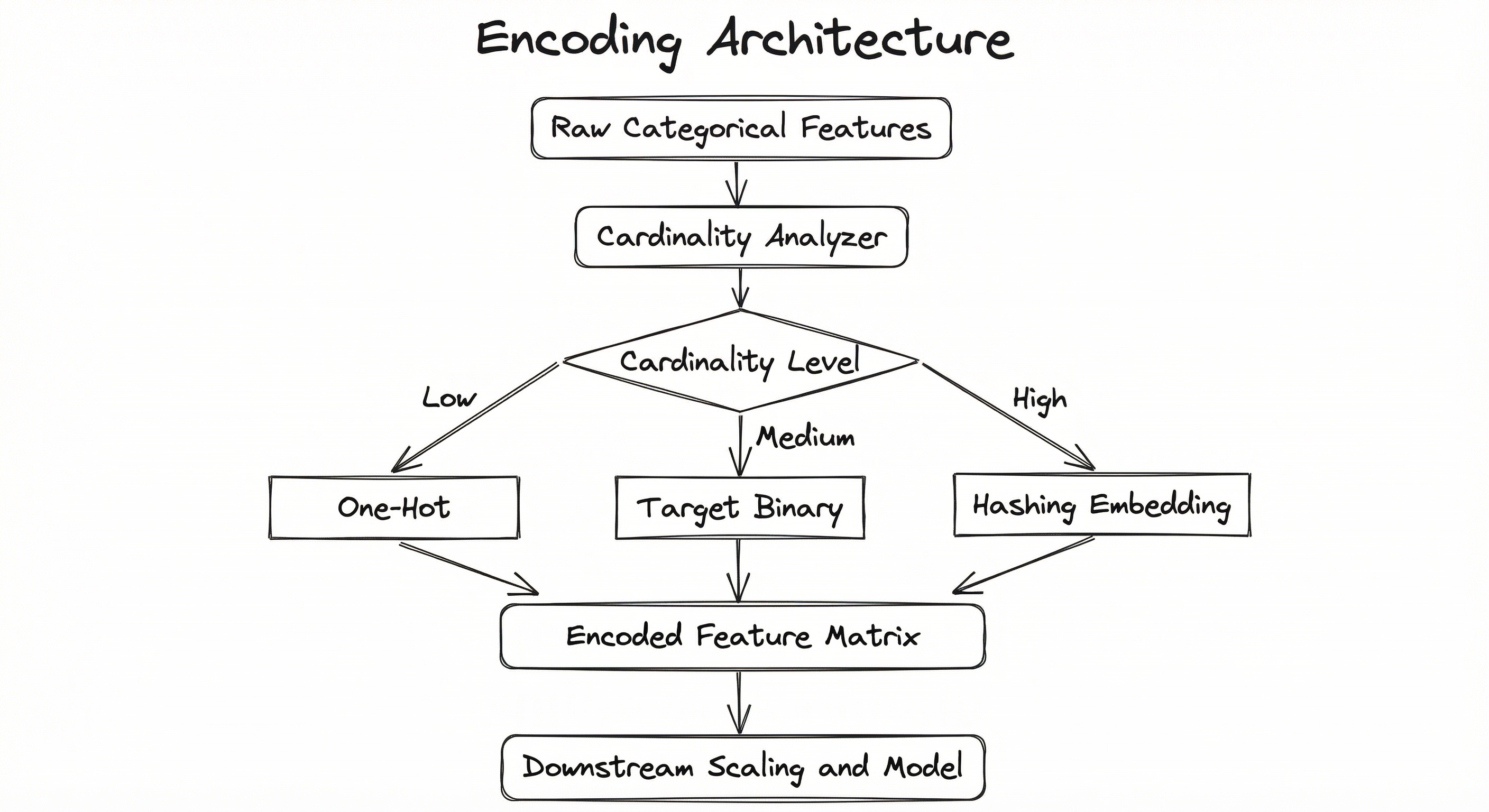
A directed flow showing raw categorical features entering a cardinality analyzer, which routes to one of three encoding paths (one-hot for low cardinality, target/binary for medium, hashing/embedding for high cardinality), all converging into an encoded feature matrix that feeds downstream scaling and model training.

How to Implement

Choosing the Right Implementation

The Python ecosystem offers three main libraries for categorical encoding, each with distinct strengths:

scikit-learn provides OneHotEncoder, OrdinalEncoder, and LabelEncoder in its preprocessing module. These are battle-tested, well-documented, and integrate seamlessly with scikit-learn pipelines. However, they lack advanced encoders like target encoding (added in v1.3+ as TargetEncoder), WoE, or CatBoost encoding.

category_encoders (scikit-learn-contrib) is the most comprehensive library, offering 20+ encoding schemes including TargetEncoder, WOEEncoder, BinaryEncoder, HashingEncoder, CatBoostEncoder, JamesSteinEncoder, and more. All encoders follow the scikit-learn transformer API (fit / transform) and work with pandas DataFrames.

feature-engine provides a curated set of encoders (OrdinalEncoder, CountFrequencyEncoder, MeanEncoder, WoEEncoder, DecisionTreeEncoder) with strong support for feature selection integration and a focus on preventing target leakage via built-in cross-validation.

For deep learning, PyTorch and TensorFlow/Keras provide nn.Embedding and tf.keras.layers.Embedding respectively -- learnable lookup tables that map integer category indices to dense vectors.

Cost Note: All three libraries are open-source and free. The computational cost of encoding is typically negligible compared to model training. For a dataset with 10M rows and 50 categorical features, encoding takes 10-60 seconds on a 4-core machine (~INR 3/hour on AWS t3.xlarge, or $0.04/hour). The real cost concern is the downstream impact on model memory: one-hot encoding 50 features with average cardinality 500 produces 25,000 columns, requiring ~2 GB RAM for 10M rows in float32.

One-Hot Encoding with scikit-learn (handling unknown categories)36 lines

import pandas as pd
from sklearn.preprocessing import OneHotEncoder
from sklearn.compose import ColumnTransformer

# Sample data: Swiggy-style restaurant features
df_train = pd.DataFrame({
    'cuisine': ['North Indian', 'Chinese', 'South Indian', 'Italian', 'North Indian'],
    'payment': ['UPI', 'Credit Card', 'Cash', 'UPI', 'Credit Card'],
    'delivery_time': [30, 45, 25, 50, 35]
})

df_test = pd.DataFrame({
    'cuisine': ['North Indian', 'Thai', 'Chinese'],  # 'Thai' unseen in train
    'payment': ['UPI', 'Cash', 'UPI'],
    'delivery_time': [28, 40, 38]
})

# Configure encoder: handle_unknown='infrequent_if_exist' groups rare/unseen categories
ohe = OneHotEncoder(
    handle_unknown='infrequent_if_exist',
    min_frequency=2,           # Categories with freq < 2 are grouped
    sparse_output=False,       # Dense array for small datasets
    drop='if_binary'           # Drop one column for binary features
)

cat_features = ['cuisine', 'payment']
preprocessor = ColumnTransformer(
    transformers=[('cat', ohe, cat_features)],
    remainder='passthrough'
)

X_train = preprocessor.fit_transform(df_train)
X_test = preprocessor.transform(df_test)  # 'Thai' mapped to infrequent category

print(f"Train shape: {X_train.shape}")  # (5, 5) - compressed from 7 categories
print(f"Test shape: {X_test.shape}")    # (3, 5) - same dimensions, no crash

This example demonstrates production-safe one-hot encoding with two critical features: handle_unknown='infrequent_if_exist' prevents crashes when unseen categories appear at inference time, and min_frequency groups rare categories to control dimensionality. The ColumnTransformer applies encoding selectively to categorical columns while passing numeric columns through unchanged -- a pattern you will use in virtually every real pipeline.

Target Encoding with regularization (category_encoders)47 lines

import pandas as pd
import numpy as np
from category_encoders import TargetEncoder
from sklearn.model_selection import KFold

# Simulate a Zomato restaurant rating prediction dataset
np.random.seed(42)
n = 10000
areas = np.random.choice(
    ['Koramangala', 'Indiranagar', 'HSR Layout', 'Whitefield',
     'Electronic City', 'Jayanagar', 'Marathahalli', 'Yelahanka',
     'Hebbal', 'Banashankari', 'JP Nagar', 'BTM Layout',
     'Malleshwaram', 'Rajajinagar', 'Basavanagudi'],
    size=n
)
ratings = np.random.uniform(2.5, 4.8, size=n)

df = pd.DataFrame({'area': areas, 'rating': ratings})

# WRONG: Fit on full data -> target leakage!
# te = TargetEncoder().fit(df[['area']], df['rating'])

# RIGHT: Use cross-validated target encoding to prevent leakage
te = TargetEncoder(
    cols=['area'],
    smoothing=10.0,        # Regularization: blend with global mean
    min_samples_leaf=20,   # Min samples before using category mean
    handle_unknown='value' # Unseen categories get global mean
)

# Cross-validated encoding for training data
kf = KFold(n_splits=5, shuffle=True, random_state=42)
df['area_encoded'] = np.nan

for train_idx, val_idx in kf.split(df):
    te.fit(df.iloc[train_idx][['area']], df.iloc[train_idx]['rating'])
    df.loc[val_idx, 'area_encoded'] = te.transform(
        df.iloc[val_idx][['area']]
    )['area'].values

# Refit on full training data for inference-time use
te.fit(df[['area']], df['rating'])

# At inference time:
new_data = pd.DataFrame({'area': ['Koramangala', 'Unknown Area']})
encoded = te.transform(new_data)
print(encoded)  # 'Unknown Area' gets global mean

Target encoding replaces each category with the mean target value for that category. The critical implementation detail is cross-validated encoding during training to prevent target leakage. Without it, the model sees its own labels during training, inflating metrics by 2-5% on typical datasets. The smoothing parameter controls how much rare categories are pulled toward the global mean -- essential when some restaurant areas in the Zomato dataset have only a handful of orders.

Binary Encoding and Feature Hashing for high-cardinality features33 lines

import pandas as pd
import numpy as np
from category_encoders import BinaryEncoder, HashingEncoder

# Simulate high-cardinality feature: Indian PIN codes
np.random.seed(42)
n = 50000
pin_codes = [f"{np.random.randint(100000, 999999)}" for _ in range(n)]
df = pd.DataFrame({'pin_code': pin_codes, 'delivery_success': np.random.binomial(1, 0.85, n)})

print(f"Unique PIN codes: {df['pin_code'].nunique()}")  # ~49,000+

# Approach 1: Binary Encoding
# For 50,000 categories: ceil(log2(50000)) = 16 columns vs 50,000 for one-hot
be = BinaryEncoder(cols=['pin_code'])
df_binary = be.fit_transform(df[['pin_code']])
print(f"Binary encoding columns: {df_binary.shape[1]}")  # 16 columns

# Approach 2: Feature Hashing (no fitting needed, handles unseen categories)
he = HashingEncoder(cols=['pin_code'], n_components=32)  # Fixed 32 buckets
df_hashed = he.fit_transform(df[['pin_code']])
print(f"Hashing encoding columns: {df_hashed.shape[1]}")  # 32 columns

# Feature hashing handles completely new PIN codes without retraining
new_pins = pd.DataFrame({'pin_code': ['999999', '123456', '000001']})
new_hashed = he.transform(new_pins)
print(f"New PIN codes encoded successfully: {new_hashed.shape}")  # (3, 32)

# Collision analysis: how many categories share a bucket?
from collections import Counter
bucket_assignments = he.transform(df[['pin_code']]).values.argmax(axis=1)
collision_rate = 1 - len(set(bucket_assignments)) / len(set(pin_codes))
print(f"Approximate collision rate: {collision_rate:.2%}")

This example contrasts two approaches for high-cardinality features like Indian PIN codes (~19,000 valid codes, but user input may produce even more unique values). Binary encoding reduces 50,000 categories to just 16 columns using binary representation -- a 3,125x compression. Feature hashing maps categories to a fixed number of buckets without any fitting step, making it ideal for streaming or online-learning scenarios where new categories appear continuously. The tradeoff is hash collisions, which introduce noise proportional to the collision rate.

Entity Embeddings with PyTorch for categorical features63 lines

import torch
import torch.nn as nn
import numpy as np

class TabularModel(nn.Module):
    """Neural network with learned embeddings for categorical features.
    
    Pattern used by Swiggy, DoorDash, and Uber for delivery time prediction.
    """
    def __init__(self, cat_dims, emb_dims, n_continuous, output_dim=1):
        super().__init__()
        
        # Create embedding layers for each categorical feature
        # Rule of thumb: emb_dim = min(50, ceil(cardinality / 2))
        self.embeddings = nn.ModuleList([
            nn.Embedding(num_categories, emb_dim)
            for num_categories, emb_dim in zip(cat_dims, emb_dims)
        ])
        
        # Total input dim = sum of embedding dims + continuous features
        total_emb_dim = sum(emb_dims)
        input_dim = total_emb_dim + n_continuous
        
        self.fc = nn.Sequential(
            nn.Linear(input_dim, 256),
            nn.ReLU(),
            nn.BatchNorm1d(256),
            nn.Dropout(0.3),
            nn.Linear(256, 128),
            nn.ReLU(),
            nn.BatchNorm1d(128),
            nn.Dropout(0.2),
            nn.Linear(128, output_dim)
        )
    
    def forward(self, x_cat, x_cont):
        # x_cat: (batch, n_cat_features) - integer indices
        # x_cont: (batch, n_continuous) - float values
        embeddings = [
            emb(x_cat[:, i]) for i, emb in enumerate(self.embeddings)
        ]
        x = torch.cat(embeddings + [x_cont], dim=1)
        return self.fc(x)


# Example: Delivery time prediction
cat_dims = [15, 500, 20000, 5]    # city, restaurant_id, area_id, payment_method
emb_dims = [8, 50, 50, 3]         # embedding dimensions per feature
n_continuous = 10                   # distance, hour, day_of_week, etc.

model = TabularModel(cat_dims, emb_dims, n_continuous)

# Dummy forward pass
batch_size = 64
x_cat = torch.randint(0, 5, (batch_size, 4))   # categorical indices
x_cont = torch.randn(batch_size, 10)            # continuous features
prediction = model(x_cat, x_cont)
print(f"Output shape: {prediction.shape}")  # (64, 1)

# Total embedding parameters:
total_params = sum(c * e for c, e in zip(cat_dims, emb_dims))
print(f"Embedding parameters: {total_params:,}")  # 1,030,135
print(f"vs One-Hot dimensions: {sum(cat_dims):,}")  # 20,520

Entity embeddings learn dense, low-dimensional representations for each category during training. This approach is standard in production deep learning systems at companies like Uber (DeepETA), DoorDash (store2vec), and Swiggy. The key advantage over one-hot encoding is dimensionality reduction (1M+ parameters vs. 20K+ sparse columns) and the ability to capture latent relationships -- for example, the model might learn that restaurant_ids serving similar cuisines have nearby embeddings. The rule of thumb for embedding dimension is $d = \min(50, \lceil k/2 \rceil)$ .

Weight of Evidence (WoE) encoding for credit risk modeling47 lines

import pandas as pd
import numpy as np
from category_encoders import WOEEncoder

# Simulate credit scoring data (common in Indian NBFC/fintech companies)
np.random.seed(42)
n = 20000

df = pd.DataFrame({
    'employment_type': np.random.choice(
        ['Salaried', 'Self-Employed', 'Business', 'Freelancer', 'Government'],
        size=n, p=[0.4, 0.2, 0.15, 0.1, 0.15]
    ),
    'education': np.random.choice(
        ['Graduate', 'Post-Graduate', 'Under-Graduate', 'Doctorate', 'Diploma'],
        size=n, p=[0.35, 0.25, 0.2, 0.05, 0.15]
    ),
    'loan_default': np.random.binomial(1, 0.12, size=n)  # 12% default rate
})

# WoE encoding: specifically designed for binary classification
woe = WOEEncoder(cols=['employment_type', 'education'], regularization=1.0)

df_encoded = woe.fit_transform(df[['employment_type', 'education']], df['loan_default'])

# Inspect the WoE values
print("WoE mapping for employment_type:")
for cat in df['employment_type'].unique():
    woe_val = df_encoded.loc[df['employment_type'] == cat, 'employment_type'].iloc[0]
    print(f"  {cat}: WoE = {woe_val:.4f}")

# Compute Information Value (IV) to assess predictive power
def compute_iv(df, feature, target):
    """IV < 0.02: useless, 0.02-0.1: weak, 0.1-0.3: medium, > 0.3: strong"""
    groups = df.groupby(feature)[target].agg(['sum', 'count'])
    groups.columns = ['events', 'total']
    groups['non_events'] = groups['total'] - groups['events']
    total_events = groups['events'].sum()
    total_non_events = groups['non_events'].sum()
    groups['pct_events'] = groups['events'] / total_events
    groups['pct_non_events'] = groups['non_events'] / total_non_events
    groups['woe'] = np.log(groups['pct_events'] / groups['pct_non_events'].clip(1e-10))
    groups['iv'] = (groups['pct_events'] - groups['pct_non_events']) * groups['woe']
    return groups['iv'].sum()

iv = compute_iv(df, 'employment_type', 'loan_default')
print(f"\nInformation Value (employment_type): {iv:.4f}")

Weight of Evidence encoding originates from credit scoring and is widely used by Indian NBFCs and fintech companies like Razorpay, Lendingkart, and Capital Float. WoE transforms each category into the log-odds ratio of positive vs. negative outcomes, creating a monotonic relationship with the logistic regression target. The companion metric Information Value (IV) quantifies the predictive power of each feature: IV < 0.02 is useless, 0.02-0.1 is weak, 0.1-0.3 is medium, and > 0.3 is strong. The regularization parameter adds Laplace smoothing to prevent infinite WoE values when a category has zero events.

CatBoost Ordered Target Encoding (built-in)52 lines

from catboost import CatBoostClassifier, Pool
import pandas as pd
import numpy as np

# CatBoost handles categorical encoding internally using Ordered Target Statistics
np.random.seed(42)
n = 5000

df = pd.DataFrame({
    'city': np.random.choice(
        ['Mumbai', 'Delhi', 'Bengaluru', 'Chennai', 'Hyderabad',
         'Pune', 'Kolkata', 'Ahmedabad', 'Jaipur', 'Lucknow'],
        size=n
    ),
    'product_category': np.random.choice(
        ['Electronics', 'Fashion', 'Groceries', 'Home', 'Beauty'],
        size=n
    ),
    'order_value': np.random.uniform(100, 5000, size=n),
    'is_returned': np.random.binomial(1, 0.15, size=n)
})

# Specify which columns are categorical -- CatBoost handles the rest
cat_features = ['city', 'product_category']

train_pool = Pool(
    data=df[['city', 'product_category', 'order_value']],
    label=df['is_returned'],
    cat_features=cat_features  # Tell CatBoost these are categorical
)

model = CatBoostClassifier(
    iterations=500,
    learning_rate=0.05,
    depth=6,
    verbose=100,
    one_hot_max_size=5,  # One-hot for features with <= 5 categories
    random_seed=42
)

model.fit(train_pool)

# CatBoost uses Ordered Target Statistics internally:
# For each observation, it computes target stats using only
# PRECEDING observations in a random permutation -- this prevents
# the target leakage that plagues naive target encoding.
print("\nFeature importance:")
for name, importance in zip(
    ['city', 'product_category', 'order_value'],
    model.feature_importances_
):
    print(f"  {name}: {importance:.2f}")

CatBoost's killer feature is its Ordered Target Statistics encoding: for each training example, it computes target statistics using only observations that precede it in a random permutation. This eliminates target leakage without requiring explicit cross-validation loops. The one_hot_max_size parameter automatically switches to one-hot encoding for low-cardinality features. This approach, introduced in the 2017 CatBoost paper by Prokhorenkova et al., consistently outperforms manual target encoding in benchmarks.

Configuration Example45 lines

# Feature engineering pipeline config (YAML)
encoding:
  features:
    - name: cuisine_type
      cardinality: 15
      method: one_hot
      params:
        handle_unknown: infrequent_if_exist
        min_frequency: 50
        drop: if_binary
    
    - name: restaurant_id
      cardinality: 250000
      method: target_encoding
      params:
        smoothing: 20.0
        min_samples_leaf: 50
        cv_folds: 5
        handle_unknown: global_mean
    
    - name: pin_code
      cardinality: 19000
      method: hashing
      params:
        n_components: 64
        hash_function: murmurhash3
    
    - name: payment_method
      cardinality: 4
      method: one_hot
      params:
        drop: first
    
    - name: product_category
      cardinality: 50000
      method: embedding
      params:
        embedding_dim: 50
        pretrained: null

  global:
    unknown_strategy: global_mean
    nan_strategy: treat_as_category
    persistence: joblib
    encoding_version: "v2.3"

Common Implementation Mistakes

●
Fitting encoders on the full dataset (train + test): This is the most common and most damaging mistake. Target encoders, WoE encoders, and even one-hot encoders must be fit exclusively on training data. Fitting on the full dataset leaks test-set information into the encoding, inflating validation metrics by 2-10% and producing models that fail in production.
●
Using label encoding for nominal features with linear models: Label encoding assigns integers (0, 1, 2, ...) that imply an ordering. For a feature like city with values {Mumbai=0, Delhi=1, Bengaluru=2}, a linear model will treat Delhi as 'between' Mumbai and Bengaluru -- meaningless. Use one-hot or target encoding instead for nominal features fed to linear/distance-based models.
●
Ignoring unseen categories at inference time: Production data will contain categories not seen during training. If your encoder crashes on unknown categories (the default behavior of many implementations), your inference pipeline fails silently or loudly. Always configure handle_unknown='value' or equivalent, and test with novel categories before deploying.
●
One-hot encoding high-cardinality features without dimensionality control: One-hot encoding a feature with 10,000+ categories creates a 10,000-column sparse matrix per feature. This bloats memory, slows training, and often hurts model performance due to the curse of dimensionality. Use target encoding, feature hashing, or embeddings for high-cardinality features.
●
Applying target encoding without regularization on rare categories: A category seen only 3 times in training data with all 3 being positive will get a target encoding of 1.0 -- pure overfitting. Always use smoothing (blend with global mean) or minimum sample thresholds. The smoothing parameter in category_encoders controls this.
●
Forgetting to encode the same way at training and inference: If you use k-fold target encoding during training but single-pass target encoding at inference, the distributions will differ. Maintain a single fitted encoder object (serialized via pickle or joblib) for both training validation and production inference.
●
Not handling NaN/missing values before encoding: Many encoders treat NaN as a valid category, silently creating a NaN bucket with its own encoding. Decide explicitly whether missing values should be a separate category or imputed before encoding.

When Should You Use This?

Use When

Your dataset contains categorical features that need to be converted to numeric form for model consumption -- which is virtually every real-world ML problem
You have low-cardinality nominal features (2-20 categories) that should be one-hot encoded to avoid imposing false ordinal relationships
You have high-cardinality features (100+ categories) like user IDs, product IDs, or ZIP codes that need compact representations via target encoding, hashing, or embeddings
You are building a credit scoring or risk model where Weight of Evidence encoding provides interpretable, monotonic transformations aligned with logistic regression
You need online-compatible encoding that handles previously unseen categories without retraining -- use feature hashing
You are training a deep learning model on tabular data and want the model to learn categorical representations end-to-end via embedding layers
You have ordinal features (e.g., education level: High School < Bachelor's < Master's < PhD) where the natural ordering should be preserved via ordinal encoding

Avoid When

Your feature is already numeric -- encoding is for categorical-to-numeric transformation only. Do not encode continuous variables (use binning/discretization instead if you want to categorize them)
The categorical feature has only 2 unique values and your model handles binary inputs natively -- a single 0/1 column suffices without a full encoding pipeline
You are using a model that handles categorical features natively (CatBoost, LightGBM with categorical_feature parameter) -- let the model handle encoding internally for optimal results
The categorical feature is a free-text field (user reviews, descriptions) -- use NLP techniques (TF-IDF, sentence embeddings) rather than categorical encoding
You have a target variable with severe class imbalance and are considering target encoding without regularization -- the encoded values for rare-class categories will be unreliable and leak noise rather than signal
The feature has extremely high cardinality with uniform distribution (e.g., unique transaction IDs) -- no encoding can extract meaningful signal from a feature where every value appears once. Drop the feature or extract derived features (e.g., transaction frequency per user)

Key Tradeoffs

The Fundamental Tradeoff: Dimensionality vs. Information Preservation

One-hot encoding preserves maximum information (each category is fully distinguishable) but at the cost of $k$ new columns. For a Flipkart product catalog with 50,000 leaf categories, this means 50,000 sparse columns per feature -- infeasible for most models and expensive in memory.

Target encoding collapses to a single column but conflates categories that happen to have similar target means. Two completely different restaurant types might get similar encodings simply because their average delivery time happens to be close.

Method	Dimensions	Leakage Risk	Unseen Categories	Best For
One-Hot	$k$	None	Needs explicit handling	Low cardinality ( $k < 20$ ), linear models
Label/Ordinal	1	None	Needs mapping	Ordinal features, tree models
Target	1	High (needs CV)	Maps to global mean	Medium-high cardinality, tree models
Binary	$\lceil \log_2 k \rceil$	None	Partial handling	Medium cardinality (20-1000)
Hashing	$m$ (fixed)	None	Automatic	Very high cardinality, streaming
WoE	1	High (needs CV)	Needs handling	Binary classification, credit scoring
Embedding	$d$ (learned)	None	Needs fallback	Deep learning, high cardinality

The Second Tradeoff: Preprocessing Simplicity vs. Model Integration

Standalone encoders (one-hot, target, binary) are model-agnostic preprocessing steps. You encode once and feed to any model. Embedding layers are tightly coupled to neural network training -- you cannot export an embedding encoding and plug it into XGBoost (though you can extract the learned embeddings post-training as features for other models, a technique called embedding transfer).

Rule of Thumb: Start simple. Use one-hot for features with $k < 20$ , target encoding with 5-fold CV for features with $20 \leq k \leq 1000$ , and embeddings or feature hashing for $k > 1000$ . Then measure the impact on your validation metric and adjust.

Alternatives & Comparisons

Feature Extraction

Feature extraction derives new numeric features from raw data (e.g., extracting day-of-week from a timestamp, or TF-IDF from text). Encoding converts existing categorical labels to numeric form. If your 'categorical' feature is actually free text or a timestamp, you need feature extraction, not encoding.

Feature Scaling / Normalization

Scaling transforms the range or distribution of already-numeric features (min-max, standard, robust scaling). Encoding converts non-numeric features to numeric. In a pipeline, encoding happens first, then scaling is applied to the encoded outputs (especially for target encoding, which produces values on the target's scale).

Data Transformation

Data transformation is a broader category that includes encoding, scaling, log transforms, and other numeric manipulations. Encoding is specifically the categorical-to-numeric conversion step within the larger transformation pipeline.

Pros, Cons & Tradeoffs

Advantages

Unlocks categorical signal for models: Without encoding, categorical features are invisible to most ML algorithms. Proper encoding surfaces the predictive signal hidden in category labels -- often the most important features in a model (e.g., merchant_category in fraud detection).
Multiple methods for different scenarios: The encoding toolbox is rich. Low-cardinality features get one-hot encoding (simple, no information loss). High-cardinality features get target encoding or embeddings (compact, high signal). This flexibility means you can optimize per-feature rather than applying a one-size-fits-all approach.
Mature ecosystem with production-ready libraries: scikit-learn, category_encoders, feature-engine, and deep learning frameworks all provide battle-tested encoding implementations. You rarely need to implement encoding from scratch.
Embeddings capture latent relationships: Entity embedding layers learn that 'Mumbai' and 'Pune' are more similar than 'Mumbai' and 'Chennai', or that 'Electronics' and 'Appliances' are related product categories. This latent structure improves model generalization beyond what one-hot encoding can achieve.
Enables model interpretability: WoE encoding produces values directly interpretable as log-odds contributions, making it a favorite in regulated industries (banking, insurance) where model explainability is a compliance requirement.
Memory efficiency at scale: Feature hashing and binary encoding reduce high-cardinality features from thousands of columns to tens, enabling training on datasets that would otherwise exceed available memory. A 50,000-category feature encoded in 16 binary columns saves ~300x memory vs. one-hot.

Disadvantages

Target leakage is a constant threat: Any encoding method that uses the target variable (target encoding, WoE, CatBoost encoding) risks leaking label information into features. Without careful cross-validation, this inflates training metrics and produces models that underperform in production by 2-10%.
Unseen categories break pipelines: Categories not present in training data cause failures at inference time unless explicitly handled. This is especially problematic in dynamic domains (new restaurants on Swiggy, new products on Flipkart) where novel categories appear daily.
One-hot encoding creates dimensionality explosion: For features with $k > 100$ categories, one-hot encoding produces prohibitively large sparse matrices. This increases training time, memory usage, and can degrade model performance due to the curse of dimensionality.
Encoding choices interact with model type: The same encoding can be optimal for one model and harmful for another. Target encoding works well for tree models but can cause multicollinearity issues in linear regression. One-hot encoding is ideal for linear models but wasteful for trees. This model-encoding interaction adds complexity to pipeline design.
Ordinal assumptions are easy to introduce accidentally: Label encoding and ordinal encoding impose a numeric ordering on categories. If the feature is nominal (no natural order), this creates a false signal that misleads linear models, KNN, and SVMs.
Maintenance burden in production: Encoding vocabularies, target statistics, and embedding weights must be versioned, persisted, and kept in sync between training and serving. Category drift (new categories appearing, old ones disappearing) requires periodic re-fitting and redeployment.

Use at least $m \geq 2k$ buckets to keep expected collision rate below 50%. Monitor collision rate empirically. Consider signed hashing (the alternate_sign parameter in scikit-learn's FeatureHasher) to reduce collision bias by making collisions cancel out in expectation rather than accumulate.

Placement in an ML System

Where Does Encoding Sit in the ML Pipeline?

Encoding occupies the feature engineering stage, immediately after data cleaning and before feature scaling/normalization and model training. In a production pipeline, encoding is typically implemented as part of a feature transformation pipeline that runs both during training and at inference time.

In a batch training pipeline (e.g., Flipkart's daily product ranking model), encoding runs as a Spark or Pandas transformation step in the ETL process, with fitted encoders stored in a feature store or model registry.

In a real-time serving pipeline (e.g., Swiggy's delivery time prediction), the fitted encoder is loaded into the serving container and applied to each incoming request. The encoding step typically adds 0.1-1ms to inference latency -- negligible compared to model inference itself.

For streaming/online learning systems (e.g., ad click prediction at Hotstar), feature hashing is preferred because it requires no pre-fitted vocabulary and handles new categories without retraining.

Key Insight: Encoding is a stateful transformation -- the encoder parameters learned during training must be applied identically at inference. This statefulness makes encoding one of the most common sources of train-serve skew in production ML systems.

Pipeline Stage

Feature Engineering / Preprocessing

Upstream

data-cleaning
exploratory-analysis
feature-extraction

Downstream

scaling
normalization
model-training
feature-store

Scaling Bottlenecks

Where Encoding Gets Tight at Scale

The primary bottleneck is memory when using one-hot encoding on high-cardinality features. A dataset with 100M rows and a single feature with 100K categories produces a 100M x 100K sparse matrix -- roughly 40 GB even in CSR format with 1 non-zero per row. Multiply by 10 such features and you are at 400 GB.

Target encoding is CPU-bound during the fitting phase: computing conditional means requires a group-by aggregation that scales as $O(n \cdot k)$ where $n$ is the number of rows and $k$ is the number of categorical features. For 100M rows and 50 features, this takes 5-15 minutes on a single machine.

Embedding layers shift the bottleneck to GPU memory: the embedding table for a feature with 10M categories and 64 dimensions requires $10M \times 64 \times 4 \text{ bytes} \approx 2.5$ GB of GPU RAM. With multiple high-cardinality features, embedding tables can consume more GPU memory than the model itself.

Some concrete numbers: encoding 50 categorical features across 10M rows takes roughly 30-90 seconds on a 4-core machine using category_encoders, costing approximately INR 0.50 (~ $0.006) on an AWS m5.xlarge instance. At 1B rows, the same operation takes 30-90 minutes and costs INR 8-25 (~$ 0.10-0.30).

Production Case Studies

WalmartRetail / E-commerce

Walmart's data science team tackled the challenge of one-hot encoding for categorical features with extremely high cardinality in their product recommendation and demand forecasting systems. They developed optimized sparse encoding pipelines that selectively apply one-hot encoding to low-cardinality features while using feature hashing and target encoding for high-cardinality attributes like store_id and product_upc.

Outcome:

Reduced feature matrix memory footprint by 85% while maintaining model accuracy within 0.3% of the full one-hot baseline, enabling training on datasets that previously exceeded cluster memory limits.

DoorDashFood Delivery

DoorDash's DeepETA model uses learned entity embeddings for high-cardinality categorical features like store_id, replacing manual encoding approaches. Each store is embedded into a dense vector (store2vec) that captures latent characteristics like preparation speed, cuisine type, and operational efficiency. The embeddings are learned jointly with the ETA prediction objective, allowing the model to discover that stores with similar operational patterns have nearby embeddings.

Outcome:

Store embeddings improved ETA prediction accuracy by 15% compared to one-hot encoding and 8% compared to target encoding, while reducing feature dimensionality from 200K+ (one-hot) to 64 (embedding dimension) per store feature.

Rossmann (Kaggle Competition)Retail

The seminal Entity Embeddings of Categorical Variables paper by Guo and Berkhahn demonstrated the power of learned embeddings on the Rossmann Store Sales Kaggle competition. The authors used embedding layers for categorical features like Store, DayOfWeek, StateHoliday, and Promo in a neural network, achieving 3rd place. Crucially, they showed that the learned embeddings captured meaningful geographic and temporal structure -- German states with similar economic profiles clustered together in embedding space.

Outcome:

Achieved 3rd place in the Kaggle competition. The learned embeddings revealed that the neural network had independently discovered geographic proximity between German states, validating that entity embeddings capture real-world latent structure.

UberTransportation / Delivery

Uber's DeepETA model embeds all categorical features (city, product type, trip type) into dense vectors as part of a deep learning architecture for arrival time prediction. The categorical embeddings are combined with bucketized continuous features and processed through a transformer-based architecture. This approach replaced hand-engineered feature encoding pipelines with end-to-end learned representations.

Outcome:

The embedding-based approach contributed to a 20% reduction in ETA prediction error compared to the previous gradient-boosted tree model that used manual target encoding for categorical features.

Tooling & Ecosystem

scikit-learn (preprocessing)

PythonOpen Source

Provides OneHotEncoder, OrdinalEncoder, LabelEncoder, and (since v1.3) TargetEncoder. The most widely used and well-documented encoding library, integrated with scikit-learn pipelines via ColumnTransformer.

category_encoders

PythonOpen Source

The most comprehensive encoding library with 20+ encoding schemes: TargetEncoder, WOEEncoder, BinaryEncoder, HashingEncoder, CatBoostEncoder, JamesSteinEncoder, LeaveOneOutEncoder, BaseNEncoder, QuantileEncoder, and more. All encoders are scikit-learn compatible transformers.

feature-engine

PythonOpen Source

Curated feature engineering library with encoding transformers (OrdinalEncoder, CountFrequencyEncoder, MeanEncoder, WoEEncoder, DecisionTreeEncoder) that include built-in safeguards against target leakage and first-class pandas DataFrame support.

CatBoost

Python / C++Open Source

Gradient boosting library with built-in Ordered Target Statistics encoding for categorical features. Handles encoding internally during training, eliminating the need for manual preprocessing. Developed by Yandex.

PyTorch nn.Embedding

Python / C++Open Source

Learnable embedding lookup table for converting integer category indices to dense vectors. The standard approach for categorical features in PyTorch-based deep learning models. Supports sparse gradients for memory-efficient training on high-cardinality features.

TensorFlow tf.keras.layers.Embedding

Python / C++Open Source

TensorFlow/Keras equivalent of PyTorch's nn.Embedding. Converts positive integer indices to dense vectors of fixed size. Supports mask_zero for variable-length sequences and integrates with TF feature columns.

Dirty-cat (skrub)

PythonOpen Source

Specialized library for encoding dirty categorical variables -- categories with typos, variations, and inconsistencies (e.g., 'Bengaluru' vs. 'Bangalore' vs. 'Bangaluru'). Provides SimilarityEncoder, GapEncoder, and MinHashEncoder that handle string similarity during encoding.

Research & References

Entity Embeddings of Categorical Variables

Guo, Berkhahn (2016)arXiv preprint

Pioneered the use of neural network embedding layers for categorical features, showing that learned embeddings capture latent structure (geographic proximity, temporal patterns) and outperform one-hot encoding on the Rossmann Kaggle competition.

CatBoost: unbiased boosting with categorical features

Prokhorenkova, Gusev, Vorobev, Dorogush, Gulin (2018)NeurIPS 2018

Introduced Ordered Target Statistics, a permutation-based target encoding that eliminates target leakage without cross-validation. Also proposed ordered boosting to address prediction shift in gradient boosting.

Regularized target encoding outperforms traditional methods in supervised machine learning with high cardinality features

Pargent, Pfisterer, Thomas, Bischl (2022)Computational Statistics

Large-scale benchmark comparing 10 encoding methods across 28 datasets. Found that regularized target encoding consistently outperformed one-hot, label, and binary encoding for high-cardinality features, especially with tree-based models.

Encoding high-cardinality string categorical variables

Cerda, Varoquaux, Kegl (2020)IEEE TKDE

Proposed similarity encoding and gap encoding for dirty categorical variables with typos and string variations. Demonstrated that string-aware encoders outperform standard methods on real-world datasets with messy category labels.

Comparative Study on the Performance of Categorical Variable Encoders in Classification and Regression Tasks

Valdez-Valenzuela, Peralta-Torres, Beltran-Martinez (2024)arXiv preprint

Evaluated 14 encoding methods across 28 datasets with 8 ML models, finding that target encoders are most suitable for tree-based models while one-hot remains competitive for linear models on low-cardinality features.

Efficient Representations for High-Cardinality Categorical Variables in Machine Learning

Various (2025)arXiv preprint

Introduces novel encoding techniques including means encoding, low-rank encoding, and multinomial logistic regression encoding for high-cardinality categorical variables, with benchmarks against traditional methods.

Interview & Evaluation Perspective

Common Interview Questions

●
How would you encode a categorical feature with 100,000 unique values for a gradient-boosted tree model?
●
What is target encoding and how do you prevent target leakage when using it?
●
When would you use one-hot encoding vs. label encoding vs. target encoding? Walk me through your decision framework.
●
How do you handle unseen categories at inference time in a production ML system?
●
Explain entity embeddings for categorical variables. When would you choose embeddings over traditional encoding?
●
What is Weight of Evidence encoding and why is it popular in credit risk modeling?
●
How would you encode categorical features differently for a linear model vs. a tree-based model?
●
What happens if you label-encode a nominal feature and feed it to a logistic regression model?

Key Points to Mention

●
The encoding method must match the model type: one-hot for linear/distance-based models, label/ordinal for tree-based models, embeddings for neural networks. This is not a preference -- it is a hard requirement that directly impacts model quality.
●
Target encoding requires cross-validated fitting during training to prevent target leakage. CatBoost's Ordered Target Statistics is the gold standard for automatic leakage prevention.
●
High-cardinality features (>100 categories) should never be one-hot encoded in production -- use target encoding with smoothing, feature hashing, or entity embeddings instead. Quantify the memory impact: $k$ categories = $k$ columns = $k \times n \times 4$ bytes.
●
Production encoders must handle unseen categories gracefully. Feature hashing handles this automatically; other encoders need explicit fallback strategies (global mean, zero vector, dedicated unknown bucket).
●
The Information Value (IV) metric from WoE encoding is a powerful feature selection tool: IV < 0.02 means the feature is useless, > 0.3 means it is a strong predictor. Mention this in credit scoring or fintech interview contexts.
●
Entity embeddings learn latent structure that one-hot encoding cannot capture. After training, embeddings can be extracted and used as features for other models (embedding transfer).

Pitfalls to Avoid

●
Claiming one-hot encoding is always the best approach -- it fails catastrophically for high-cardinality features and is wasteful for tree models that can handle integer indices directly.
●
Forgetting to mention target leakage when discussing target encoding -- this is the single most important implementation detail and interviewers specifically listen for it.
●
Confusing label encoding with ordinal encoding -- label encoding assigns arbitrary integers, ordinal encoding assigns integers based on a meaningful order. The distinction matters for model interpretation.
●
Not addressing the production concern of unseen categories -- every interviewer who has built a real system will ask about this, and saying 'it won't happen' is a red flag.
●
Overlooking the interaction between encoding and downstream components like feature scaling. Target-encoded values are on the target's scale and may need standardization, while one-hot values are already 0/1.

Senior-Level Expectation

A senior candidate should discuss encoding as part of a holistic feature engineering strategy, not in isolation. They should articulate the cardinality-based decision framework (one-hot for low, target/binary for medium, hashing/embeddings for high), explain the mathematical basis of target leakage and how cross-validation mitigates it, and describe production concerns: encoder serialization, versioning, handling category drift, and train-serve consistency. They should mention embedding transfer (training embeddings in a neural network and exporting them for use in tree models) as a technique for combining the best of both worlds. For Indian fintech contexts, demonstrating familiarity with WoE encoding, Information Value, and RBI regulatory requirements for model interpretability would be impressive. Cost-aware analysis is expected: quantifying the memory and compute tradeoffs of different encoding approaches at the company's data scale (e.g., 'at 100M rows, one-hot encoding this 50K-cardinality feature would require 20 TB in dense form, costing approximately INR 1.5 lakh/month in cloud RAM').

Summary

Wrapping Up: The Encoding Decision Framework

Encoding is the process of converting categorical features into numerical representations that ML models can consume. While it sounds like a simple mapping exercise, the choice of encoding method has cascading effects on model accuracy, memory usage, training speed, and production reliability.

The key methods form a spectrum from simple to sophisticated:

One-hot encoding: Maximum information preservation, $k$ output dimensions. Best for low-cardinality features ( $k < 20$ ) and linear/distance-based models. The default choice when cardinality permits.
Label / ordinal encoding: Minimal dimensionality (1 column), but implies ordering. Safe for tree-based models, dangerous for linear models on nominal features.
Target encoding: Compresses any cardinality to 1 column using target statistics. Powerful but risky -- requires cross-validated fitting to prevent target leakage. The go-to method for high-cardinality features in tree-based pipelines.
Binary / Base-N encoding: Logarithmic compression ( $\lceil \log_2 k \rceil$ columns). A middle ground between one-hot and label encoding, useful for medium cardinality.
Feature hashing: Fixed-size output, stateless, handles unseen categories. Best for streaming systems and very high cardinality at the cost of collision noise.
WoE encoding: Log-odds ratio for binary classification. Standard in credit scoring and regulated industries where interpretability is mandatory.
Entity embeddings: Learned dense representations via neural networks. The state-of-the-art for high-cardinality features in deep learning systems, capable of discovering latent structure.

The decision framework is straightforward: match the encoding method to your cardinality (low/medium/high), model type (tree/linear/neural), and operational constraints (streaming, unseen categories, interpretability). Always prevent target leakage via cross-validated fitting, always handle unseen categories explicitly, and always serialize your fitted encoder for production consistency.

Bottom line: Encoding is not a one-size-fits-all step. The best ML engineers apply different encoding strategies per feature based on cardinality and model type, prevent target leakage with cross-validation, and design for the production realities of unseen categories and train-serve consistency. Get this right, and you have a solid foundation for everything downstream.

Concept Snapshot

Why This Concept Exists

The Fundamental Problem: Models Speak Numbers, Data Speaks Categories

The Evolution of Encoding Techniques

Core Intuition & Mental Model

The Core Question Every Encoding Answers

The Three Axes of Tradeoff

A Useful Mental Model

Technical Foundations

Mathematical Framework

One-Hot Encoding

Label / Ordinal Encoding

Target Encoding (Mean Encoding)

Weight of Evidence (WoE)

Binary Encoding

Feature Hashing

Entity Embedding

Internal Architecture

Key Components

Data Flow

How to Implement

Choosing the Right Implementation

Common Implementation Mistakes

When Should You Use This?

Use When

Avoid When

Key Tradeoffs

The Fundamental Tradeoff: Dimensionality vs. Information Preservation

The Second Tradeoff: Preprocessing Simplicity vs. Model Integration

Alternatives & Comparisons

Pros, Cons & Tradeoffs

Advantages

Disadvantages

Failure Modes & Debugging

Target leakage via naive target encoding

Unseen category crash at inference

Dimensionality explosion from one-hot encoding

Train-serve encoding skew

Silent ordinal injection in nominal features

Hash collision noise in feature hashing

Placement in an ML System

Where Does Encoding Sit in the ML Pipeline?

Pipeline Stage

Upstream

Downstream

Scaling Bottlenecks

Production Case Studies

Tooling & Ecosystem

Research & References

Interview & Evaluation Perspective

Common Interview Questions

Key Points to Mention

Pitfalls to Avoid

Senior-Level Expectation

Summary

Wrapping Up: The Encoding Decision Framework

Related Blocks & Further Reading

Related ML Blocks

Further Reading