Qdrant in Machine Learning
Qdrant (pronounced "quadrant") is an open-source, high-performance vector similarity search engine and database written entirely in Rust. In the rapidly growing landscape of vector databases, Qdrant has carved out a distinctive position by combining the memory safety and raw speed of Rust with a thoughtfully designed feature set that includes filterable HNSW indexing, multiple quantization strategies, native sparse vector support, and a first-class recommendation API.
With over 27,000 GitHub stars and backing from enterprises like Tripadvisor, HubSpot, Sprinklr, and Dailymotion, Qdrant has graduated from a promising newcomer to a production-grade vector database powering billions of vectors in real-world deployments. Its architecture -- built around segments, write-ahead logging, and Raft-based distributed consensus -- reflects engineering decisions that prioritize both throughput and operational reliability.
Why should you care about Qdrant specifically when there are half a dozen vector databases to choose from? Three reasons: (1) its filterable HNSW implementation solves the metadata filtering problem that plagues most vector databases, (2) its Rust foundation delivers predictable latency without garbage collection pauses, and (3) its tiered multi-tenancy model makes it particularly well-suited for SaaS applications where hundreds or thousands of tenants share a single cluster. Whether you are building a RAG pipeline for an Indian fintech startup or a recommendation engine for a global media platform, Qdrant deserves serious consideration as your vector storage layer.
Concept Snapshot
- What It Is
- An open-source vector similarity search engine written in Rust, purpose-built for storing, indexing, and querying high-dimensional vectors with rich payload filtering and quantization support.
- Category
- Vector Databases
- Complexity
- Intermediate
- Inputs / Outputs
- Inputs: dense vectors (1-65535 dimensions), sparse vectors, multi-vectors, and JSON payloads. Outputs: ranked list of nearest neighbor points with similarity scores and payloads.
- System Placement
- Sits between the embedding model (upstream) and the re-ranker, context assembler, or recommendation scorer (downstream) in RAG, search, and recommendation pipelines.
- Also Known As
- Qdrant DB, Qdrant Vector Database, Qdrant Vector Search Engine
- Typical Users
- ML Engineers, Backend Engineers, Data Engineers, Search/Retrieval Specialists, AI Application Developers
- Prerequisites
- Embeddings and vector representations, Distance metrics (cosine, L2, dot product), HNSW algorithm basics, REST/gRPC API concepts
- Key Terms
- HNSWfilterable HNSWscalar quantizationbinary quantizationproduct quantizationcollectionpointpayloadsegmentshardreplicaWALnamed vectorssparse vectorsRaft consensus
Why This Concept Exists
The Gap Between ANN Libraries and Production Databases
By 2021, the ML ecosystem had excellent ANN index libraries -- FAISS from Meta, HNSWlib from Yashunin, ScaNN from Google. But these libraries operated as in-process data structures. They had no persistence layer, no replication, no metadata filtering, and no API server. If you wanted to use FAISS in production, you had to build all of that plumbing yourself: a REST server, a write-ahead log, a snapshot mechanism, a way to handle concurrent reads and writes. Most teams ended up building a fragile, custom vector service on top of FAISS and spending more time maintaining the wrapper than tuning the index.
Qdrant was created to fill this gap -- not by wrapping an existing library but by building a purpose-designed vector database from scratch in Rust. The choice of Rust was deliberate: it provides C/C++ level performance with memory safety guarantees, zero-cost abstractions, and no garbage collector. This last point matters more than people realize. In Java-based or Go-based systems, garbage collection pauses can cause unpredictable latency spikes -- exactly what you do not want in a real-time retrieval system serving user-facing queries.
The Filtering Problem
One of the most persistent pain points with early vector databases was the interaction between vector similarity search and metadata filtering. Consider a multi-tenant RAG system where each query must retrieve documents belonging only to the querying user's workspace. The naive approach -- run ANN search first, then filter results by tenant ID -- can return fewer than results when the tenant's documents are a small fraction of the total corpus. The alternative -- filter first, then search only within matching documents -- requires building separate indices per filter combination, which is combinatorially explosive.
Qdrant's filterable HNSW implementation addresses this head-on. It extends the HNSW graph with additional edges conditioned on payload values, ensuring that the graph remains navigable even under restrictive filter predicates. This means you get both vector similarity and metadata filtering in a single graph traversal -- no pre-filtering starvation, no post-filtering misses. This was a genuine architectural innovation, not just a marketing feature.
From Niche to Mainstream
Qdrant's trajectory mirrors the broader explosion of vector database adoption driven by the RAG paradigm. When ChatGPT popularized LLM-powered applications in late 2022, every team building an AI product suddenly needed a vector database. Qdrant was well-positioned: it was already open-source, had a clean API, supported Docker deployment in minutes, and offered a managed cloud service. By 2025, Qdrant had surpassed 27,000 GitHub stars and was being used by enterprises including Tripadvisor (1B+ reviews indexed), HubSpot (powering Breeze AI), Sprinklr (enterprise CX platform), and Dailymotion (420M+ videos).
Key Takeaway: Qdrant exists because production vector search requires more than an ANN algorithm -- it requires persistence, filtering, replication, and operational tooling. Qdrant provides all of this in a single, Rust-based binary with predictable performance characteristics.
Core Intuition & Mental Model
The Rust Advantage: Predictable Speed
Here is the mental model I use for Qdrant: imagine a library with an extremely fast, never-sleeping librarian who speaks geometry. You hand the librarian a description (your query vector), and within milliseconds, the librarian navigates a network of interconnected bookshelves (the HNSW graph) to find the most similar books. But here is what makes this librarian special -- they can simultaneously check tags on each book (payload filtering) as they navigate, without slowing down. And because this librarian is built in Rust, they never pause to "take a break" (no garbage collection pauses), giving you consistent sub-10ms response times.
The Rust foundation is not just a marketing talking point. In garbage-collected runtimes (Java, Go, Python), periodic GC pauses can cause P99 latency to spike 10-50x above the median. For a vector database serving user-facing queries, a 200ms spike on a 5ms median query is unacceptable. Qdrant's Rust implementation eliminates this entire class of latency variance. When Sprinklr benchmarked Qdrant against Elasticsearch, they found Qdrant delivered P99 latency of 20ms on 1 million vectors -- consistently.
Points, Payloads, and Collections
Qdrant's data model is refreshingly simple. The core abstraction is a point -- a combination of a vector (or multiple named vectors), a JSON payload, and a unique ID. Points live in collections, which are analogous to tables in a relational database. Each collection has a fixed vector configuration (dimensions, distance metric) but accepts arbitrary JSON payloads.
This design means you store your embeddings and their metadata together, query them together, and filter on both simultaneously. No joins, no separate metadata stores, no impedance mismatch. For an Indian e-commerce company like Myntra building a visual search feature, a single point might contain an image embedding, a product category, a price range, and an availability flag -- all queryable in one call.
Why "Approximate" Is Good Enough
Like all vector databases, Qdrant uses approximate nearest neighbor (ANN) search. The word "approximate" can be unsettling, but here is the reality: for most ML applications, a recall@10 of 0.95-0.99 is indistinguishable from exact search in terms of downstream task quality. The speedup, however, is enormous -- from brute-force to graph traversal. Qdrant gives you knobs (ef parameter in HNSW) to dial the recall-speed tradeoff to exactly the level your application needs.
Technical Foundations
Mathematical Foundation
Qdrant implements vector search over a collection where each point consists of a unique identifier, a vector , and a JSON metadata payload .
Core Search Operation
Given a query vector , an optional filter predicate over payloads, and a result count , Qdrant returns:
where is one of the supported distance functions.
Supported Distance Metrics
Qdrant supports four distance metrics:
-
Cosine similarity: . Normalized to internally (Qdrant stores pre-normalized vectors and uses dot product for speed).
-
Dot product (Inner Product): . Use when vector magnitudes carry information (e.g., popularity-weighted embeddings).
-
Euclidean (L2): . Lower distance means higher similarity.
-
Manhattan (L1): . Added in recent versions for specific use cases.
HNSW Complexity
The HNSW index provides:
- Search complexity: average case, where is the number of points
- Insert complexity: per point (amortized)
- Space complexity: bytes, where is the number of connections per node and is the vector dimension
The key tuning parameters are:
- (
m): Number of bidirectional links per node. Higher increases recall and memory. Default: 16. - : Size of the dynamic candidate list during index construction. Higher values produce a higher-quality graph. Default: 100.
- (
ef): Size of the dynamic candidate list during search. Controls the recall-speed tradeoff at query time.
Quantization Memory Savings
Qdrant supports multiple quantization strategies with different compression ratios:
- Scalar quantization: Maps each float32 to uint8, achieving 4x compression. Memory per vector: bytes.
- Binary quantization: Maps each float32 to 1 bit, achieving 32x compression. Memory per vector: bytes. Works best with high-dimensional embeddings (1536+) from models like OpenAI
text-embedding-3-large. - Product quantization: Divides the vector into sub-vectors and quantizes each to a codebook index, achieving variable compression (typically 8-64x).
The memory formula for a quantized collection with vectors of dimension :
For example, 10 million 1536-dimensional vectors with binary quantization: GB -- compared to GB uncompressed. That is a 32x reduction.
Practical Note: Binary quantization with rescoring (where the full-precision vectors are used to re-rank the top candidates from the quantized search) achieves near-lossless recall while retaining most of the speed and memory benefits. Qdrant supports this out of the box with the
always_ram: trueandrescore: trueconfiguration options.
Internal Architecture
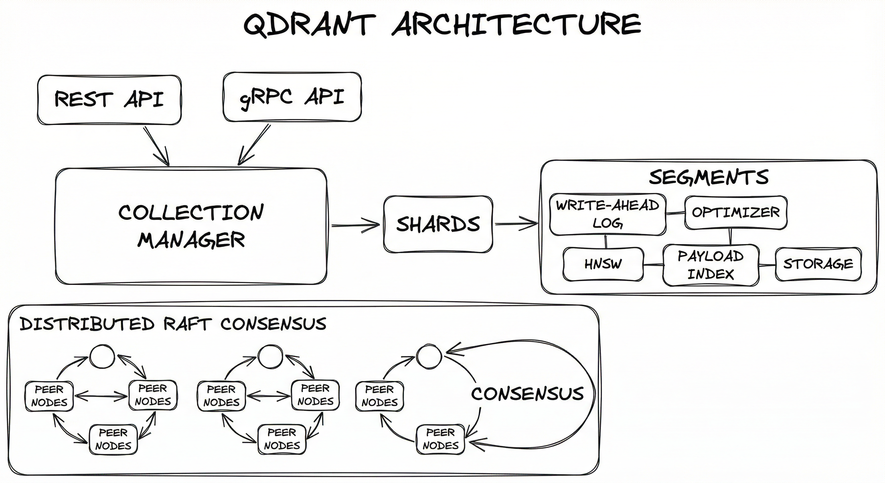
Qdrant's architecture is organized around four key layers: an API layer (REST + gRPC), a collection manager that handles data routing, a segment-based storage engine with write-ahead logging, and an optional distributed consensus layer using Raft. Let's walk through how data flows through each.
The write path begins when a client sends an upsert request via REST or gRPC. The API layer validates the request and routes it to the appropriate collection. The collection manager identifies the target shard (based on point ID hashing or custom sharding key), writes the operation to the WAL for durability, and inserts the point into an appendable segment. Background optimizers periodically merge small segments into larger, HNSW-indexed segments for query efficiency.
The read path is simpler: the query enters the API layer, fans out to all relevant shards in the collection, each shard searches its segments (both appendable and optimized) using the HNSW index with optional payload filtering, and results are merged and returned. In distributed mode, the coordinating node aggregates results from remote shards before returning the final top-k.
Key Components
API Layer (REST + gRPC)
Exposes dual APIs -- REST on port 6333 (via Actix-web) and gRPC on port 6334 (via Tonic). REST is convenient for development and debugging; gRPC is recommended for production workloads requiring maximum throughput. Both APIs support all operations: CRUD on collections and points, search, recommend, and cluster management.
Collection Manager
Manages the lifecycle of collections (create, delete, alias, update configuration). Routes operations to the correct shard based on the point ID or custom sharding key. Handles collection-level configuration like vector parameters, HNSW config, quantization settings, and replication factor.
Shards
Each collection is divided into one or more shards. By default, the number of shards equals the number of cluster nodes, but this can be configured manually. Shards can be local (on the current node) or remote (replicated to other nodes). Custom sharding keys allow routing points to specific shards -- essential for tiered multi-tenancy.
Segments
The fundamental storage unit within a shard. Each segment contains vector storage, payload storage, an HNSW index (for optimized segments), payload indices, and an ID mapper. Segments come in two flavors: appendable (accepts new writes, uses a flat/simple index) and optimized (read-only, HNSW-indexed, possibly quantized). The optimizer converts appendable segments into optimized segments in the background.
Write-Ahead Log (WAL)
All write operations are first recorded in the WAL before being applied to segments. This ensures durability -- if a crash occurs before segment flush, operations can be replayed from the WAL. The WAL is configurable in terms of segment size (default 32 MB) and pre-allocated segments.
HNSW Index Engine
Builds and maintains the hierarchical navigable small world graph for each optimized segment. Supports Qdrant's filterable HNSW extension, which adds payload-conditioned edges to maintain graph connectivity under filter predicates. Configurable via m (connections per node), ef_construct (construction quality), and ef (search quality) parameters.
Payload Index Engine
Builds inverted indices on payload fields for fast filtering. Supports multiple field types: keyword (exact match), integer/float (range queries), geo (radius/bounding box), datetime, text (full-text with tokenization), and bool. The is_tenant flag on keyword indices activates optimized storage co-location for multi-tenant workloads.
Optimizer
Runs background processes that merge small segments, build HNSW indices, apply quantization, and vacuum deleted points. Three optimizer types: merge optimizer (combines small segments), indexing optimizer (builds HNSW when segment exceeds threshold), and vacuum optimizer (cleans up deleted vectors).
Storage Backend (Gridstore)
Qdrant's custom key-value store called Gridstore provides the underlying storage for vectors, payloads, and index data. Supports in-memory and memory-mapped (mmap) modes. Gridstore uses sequential integer IDs as array-indexed pointers for O(1) lookups, making it significantly faster than general-purpose KV stores like RocksDB for Qdrant's access patterns.
Distributed Consensus (Raft)
In multi-node deployments, Qdrant uses the Raft consensus protocol to maintain consistency of cluster topology and collection metadata. Point-level operations (upsert, delete, search) bypass Raft for performance -- they are routed directly to the appropriate shard replicas. Raft ensures that all nodes agree on which shards exist, where they live, and what their configuration is.
Data Flow
- Client sends an upsert request (REST or gRPC) with point ID, vector(s), and optional payload
- API layer validates dimensions, data types, and routes to the Collection Manager
- Collection Manager identifies the target shard (via consistent hashing on point ID or custom shard key)
- The operation is written to the WAL for durability
- The point is inserted into the shard's current appendable segment
- Background optimizer periodically converts appendable segments into optimized segments with HNSW indices
- Client sends a search request with query vector, optional filter, and limit
- API layer routes to the Collection Manager
- Collection Manager fans out the query to all shards in the collection
- Each shard searches all its segments (both appendable and optimized) in parallel
- Within each optimized segment, the filterable HNSW index traverses the graph while applying payload filter predicates
- Results from all segments within a shard are merged locally
- Results from all shards are merged at the coordinating node
- Final top- results are returned to the client with scores and payloads
In a multi-node cluster, step 3 involves network RPCs to remote nodes hosting shard replicas. Qdrant supports configurable read consistency levels: 1 (fastest, read from any replica), majority (read from quorum), or all (strongest consistency, highest latency).
The architecture diagram shows a Qdrant node receiving requests via REST (port 6333) and gRPC (port 6334) APIs. Requests flow through the Collection Manager to shards, each containing multiple segments. A Write-Ahead Log ensures durability, while a background optimizer converts appendable segments into HNSW-indexed optimized segments. The storage backend (Gridstore) persists data either in-memory or via mmap. In distributed mode, a Raft consensus layer coordinates cluster topology with peer nodes.
How to Implement
Getting Started: Docker to Production
Qdrant is remarkably easy to get running. A single Docker command gives you a fully functional vector database in seconds:
docker run -p 6333:6333 -p 6334:6334 qdrant/qdrant
From there, you interact via the REST API on port 6333, gRPC on port 6334, or one of the official client SDKs (Python, TypeScript/JavaScript, Rust, Go, Java, C#). The Python client (qdrant-client) is by far the most popular and supports both REST and gRPC backends.
For production deployments, you have three options: self-hosted (Docker/Kubernetes), Qdrant Cloud (fully managed, available on AWS, GCP, and Azure), or Hybrid Cloud (Qdrant's control plane managing your infrastructure). Qdrant Cloud offers a generous free tier -- 1 GB cluster, no credit card required -- making it the lowest-friction way to start.
Key Implementation Patterns
The most common patterns when working with Qdrant are: (1) basic CRUD + search for RAG pipelines, (2) named vectors for multi-model or hybrid dense+sparse search, (3) payload-filtered multi-tenant search for SaaS applications, and (4) recommendation API for discovery and personalization. Let's look at concrete, runnable code for each.
from qdrant_client import QdrantClient
from qdrant_client.models import (
    Distance, VectorParams, PointStruct,
    Filter, FieldCondition, MatchValue,
    ScalarQuantizationConfig, ScalarType,
    OptimizersConfigDiff, HnswConfigDiff,
)
import numpy as np

# Connect to local Qdrant instance
client = QdrantClient(host="localhost", port=6333)

# Create a collection with HNSW tuning and scalar quantization
client.create_collection(
    collection_name="products",
    vectors_config=VectorParams(
        size=768,
        distance=Distance.COSINE,
        on_disk=False,  # keep vectors in RAM for speed
    ),
    hnsw_config=HnswConfigDiff(
        m=16,                # connections per node
        ef_construct=128,    # construction quality
    ),
    quantization_config=ScalarQuantizationConfig(
        type=ScalarType.INT8,
        quantile=0.99,       # clip outliers at 99th percentile
        always_ram=True,     # keep quantized vectors in RAM
    ),
    optimizers_config=OptimizersConfigDiff(
        indexing_threshold=20000,  # build HNSW after 20k points
    ),
)

# Create payload index for filtering
client.create_payload_index(
    collection_name="products",
    field_name="category",
    field_schema="keyword",
)

# Upsert points with vectors and payloads
points = [
    PointStruct(
        id=1,
        vector=np.random.rand(768).tolist(),
        payload={"category": "electronics", "price": 24999, "brand": "Samsung"},
    ),
    PointStruct(
        id=2,
        vector=np.random.rand(768).tolist(),
        payload={"category": "fashion", "price": 1299, "brand": "Zara"},
    ),
]
client.upsert(collection_name="products", points=points)

# Search with metadata filter
query_vector = np.random.rand(768).tolist()
results = client.query_points(
    collection_name="products",
    query=query_vector,
    query_filter=Filter(
        must=[FieldCondition(key="category", match=MatchValue(value="electronics"))]
    ),
    limit=10,
    with_payload=True,
)

for point in results.points:
    print(f"ID: {point.id}, Score: {point.score:.4f}, Payload: {point.payload}")
This example covers the full lifecycle: creating a collection with HNSW tuning and scalar quantization enabled, creating a payload index for efficient filtering, upserting points with embeddings and metadata, and performing a filtered similarity search. The ScalarQuantizationConfig reduces memory by 4x while typically maintaining >99% recall. The always_ram=True setting keeps quantized vectors in RAM for search while full-precision vectors can be stored on disk for rescoring.
from qdrant_client import QdrantClient, models
import numpy as np

client = QdrantClient(host="localhost", port=6333)

# Create collection with both dense and sparse named vectors
client.create_collection(
    collection_name="documents",
    vectors_config={
        "dense": models.VectorParams(
            size=1024,
            distance=models.Distance.COSINE,
        ),
    },
    sparse_vectors_config={
        "sparse": models.SparseVectorParams(
            modifier=models.Modifier.IDF,  # apply IDF weighting
        ),
    },
)

# Upsert with both dense and sparse vectors
client.upsert(
    collection_name="documents",
    points=[
        models.PointStruct(
            id=1,
            vector={
                "dense": np.random.rand(1024).tolist(),
                "sparse": models.SparseVector(
                    indices=[100, 500, 1200, 3500],  # token IDs
                    values=[0.8, 0.4, 0.9, 0.3],     # BM25/SPLADE weights
                ),
            },
            payload={"source": "arxiv", "title": "Attention Is All You Need"},
        ),
    ],
)

# Hybrid search using the Query API with Reciprocal Rank Fusion
results = client.query_points(
    collection_name="documents",
    prefetch=[
        models.Prefetch(
            query=np.random.rand(1024).tolist(),
            using="dense",
            limit=20,
        ),
        models.Prefetch(
            query=models.SparseVector(
                indices=[100, 500, 3500],
                values=[0.8, 0.4, 0.3],
            ),
            using="sparse",
            limit=20,
        ),
    ],
    query=models.FusionQuery(fusion=models.Fusion.RRF),  # Reciprocal Rank Fusion
    limit=10,
)

for point in results.points:
    print(f"ID: {point.id}, Score: {point.score:.4f}")
This demonstrates Qdrant's named vectors feature for hybrid search. Each point stores both a dense embedding (from a model like text-embedding-3-large) and a sparse vector (from BM25 or SPLADE). The Query API's prefetch mechanism runs both searches independently and fuses results using Reciprocal Rank Fusion (RRF). The IDF modifier on sparse vectors applies inverse document frequency weighting automatically. This pattern is essential for production search systems where pure semantic search misses keyword-specific queries (e.g., searching for an Indian PIN code like "560001").
from qdrant_client import QdrantClient, models
import numpy as np

client = QdrantClient(host="localhost", port=6333)

# Create collection optimized for multi-tenancy
client.create_collection(
    collection_name="rag_docs",
    vectors_config=models.VectorParams(
        size=1536,
        distance=models.Distance.COSINE,
    ),
    hnsw_config=models.HnswConfigDiff(
        payload_m=16,  # extra connections for payload-conditioned graph
    ),
)

# Create tenant index with is_tenant flag for optimized storage co-location
client.create_payload_index(
    collection_name="rag_docs",
    field_name="tenant_id",
    field_schema=models.KeywordIndexParams(
        type=models.KeywordIndexType.KEYWORD,
        is_tenant=True,  # enables storage optimization for multi-tenancy
    ),
)

# Upsert documents for different tenants
for tenant in ["flipkart", "swiggy", "razorpay"]:
    points = [
        models.PointStruct(
            id=hash(f"{tenant}_{i}") % (2**63),
            vector=np.random.rand(1536).tolist(),
            payload={
                "tenant_id": tenant,
                "doc_type": "policy",
                "content": f"Document {i} for {tenant}",
            },
        )
        for i in range(100)
    ]
    client.upsert(collection_name="rag_docs", points=points)

# Search scoped to a single tenant
results = client.query_points(
    collection_name="rag_docs",
    query=np.random.rand(1536).tolist(),
    query_filter=models.Filter(
        must=[
            models.FieldCondition(
                key="tenant_id",
                match=models.MatchValue(value="razorpay"),
            )
        ]
    ),
    limit=5,
    with_payload=True,
)

print(f"Results for tenant 'razorpay':")
for point in results.points:
    print(f"  ID: {point.id}, Score: {point.score:.4f}")
This pattern is critical for SaaS RAG applications. The is_tenant=True flag on the payload index tells Qdrant to co-locate vectors belonging to the same tenant in storage, dramatically improving filtered search performance. Qdrant's filterable HNSW ensures that even tenants with very few documents (say, a small startup using your platform) get accurate results -- the graph traversal adapts to the filter, unlike post-filtering which would starve small tenants. For Indian SaaS companies building multi-tenant AI features -- think Zoho, Freshworks, or Razorpay -- this is the recommended architecture.
from qdrant_client import QdrantClient, models

client = QdrantClient(host="localhost", port=6333)

# Assume 'movies' collection exists with movie embeddings
# Recommend movies similar to liked ones, dissimilar from disliked ones
results = client.recommend(
    collection_name="movies",
    positive=[42, 107, 238],   # point IDs of liked movies
    negative=[15, 89],          # point IDs of disliked movies
    strategy=models.RecommendStrategy.AVERAGE_VECTOR,
    query_filter=models.Filter(
        must=[
            models.FieldCondition(
                key="language",
                match=models.MatchValue(value="hindi"),
            ),
            models.FieldCondition(
                key="year",
                match=models.MatchValue(value=2025),
            ),
        ]
    ),
    limit=10,
    with_payload=True,
)

print("Recommended Hindi movies from 2025:")
for point in results:
    print(f"  {point.payload.get('title', 'Unknown')} (Score: {point.score:.4f})")

# Discovery API: explore a region of vector space
# constrained by context pairs
discovery_results = client.discover(
    collection_name="movies",
    target=42,  # point ID to search near
    context=[
        models.ContextExamplePair(
            positive=107,  # prefer this direction
            negative=15,   # avoid this direction
        ),
    ],
    limit=10,
)
Qdrant's Recommend API is unique among vector databases. Instead of providing a query vector, you provide point IDs of positive (liked) and negative (disliked) examples. Qdrant computes an aggregate query internally using either AVERAGE_VECTOR (centroid of positives minus negatives) or BEST_SCORE (max similarity across all positive examples). The Discovery API goes further -- it defines a target direction and context constraints to explore specific regions of the vector space. This is perfect for building recommendation systems like a Hotstar content recommender or a Flipkart product discovery feature where users interactively refine their preferences.
from qdrant_client import QdrantClient
import requests

client = QdrantClient(host="localhost", port=6333)

# Create a snapshot of a collection
snapshot_info = client.create_snapshot(collection_name="products")
print(f"Snapshot created: {snapshot_info.name}")

# List all snapshots
snapshots = client.list_snapshots(collection_name="products")
for snap in snapshots:
    print(f"  {snap.name} | Size: {snap.size} bytes | Created: {snap.creation_time}")

# Download snapshot (via REST API)
snapshot_name = snapshot_info.name
url = f"http://localhost:6333/collections/products/snapshots/{snapshot_name}"
response = requests.get(url, stream=True)
with open(f"/backups/{snapshot_name}", "wb") as f:
    for chunk in response.iter_content(chunk_size=8192):
        f.write(chunk)
print(f"Snapshot downloaded to /backups/{snapshot_name}")

# Restore from snapshot (upload to a new or existing collection)
# Using REST API for restore
with open(f"/backups/{snapshot_name}", "rb") as f:
    response = requests.post(
        "http://localhost:6333/collections/products_restored/snapshots/upload",
        files={"snapshot": f},
    )
print(f"Restore status: {response.status_code}")

# Full storage snapshot (all collections)
full_snapshot = client.create_full_snapshot()
print(f"Full snapshot created: {full_snapshot.name}")
Snapshots are Qdrant's mechanism for backup and restore. They are complete tarballs containing all data, indices, and configuration needed to restore a collection. You can snapshot individual collections or the entire storage. This is essential for disaster recovery, migration between environments, and blue-green reindexing workflows. For regulated industries in India (BFSI, healthcare), regular snapshot schedules should be part of your compliance checklist.
# Qdrant production configuration (config.yaml)
service:
  host: 0.0.0.0
  http_port: 6333
  grpc_port: 6334
  enable_tls: true
  api_key: "${QDRANT_API_KEY}"  # Use environment variable

storage:
  storage_path: /data/qdrant/storage
  snapshots_path: /data/qdrant/snapshots

  # WAL configuration
  wal:
    wal_capacity_mb: 64
    wal_segments_ahead: 1

  # Optimizer configuration
  optimizers:
    deleted_threshold: 0.2      # vacuum when 20% of points are deleted
    vacuum_min_vector_number: 1000
    default_segment_number: 2
    indexing_threshold: 20000   # build HNSW after 20k points
    flush_interval_sec: 5

  # HNSW defaults for new collections
  hnsw_index:
    m: 16
    ef_construct: 128
    full_scan_threshold: 10000  # brute-force if fewer points match filter

  # Performance tuning
  performance:
    max_search_threads: 0       # 0 = auto (num CPUs)
    max_optimization_threads: 2

# Cluster configuration (for distributed mode)
cluster:
  enabled: true
  p2p:
    port: 6335
  consensus:
    tick_period_ms: 100
Common Implementation Mistakes
- ●
Using gRPC with large payloads without benchmarking: Counterintuitively, gRPC can be slower than REST when payloads contain large strings due to protobuf serialization overhead. A GitHub issue showed REST at 60ms vs. gRPC at 226ms for batch queries with large payloads. Always benchmark both protocols with your actual data before committing to gRPC.
- ●
Skipping payload index creation for filter fields: Without a payload index, Qdrant falls back to brute-force scanning of payloads during filtering. For a collection with millions of points, this turns a 5ms query into a 500ms query. Always create payload indices on fields you filter by, especially
tenant_id. - ●
Not setting
is_tenant: truefor multi-tenant deployments: Without the tenant flag, Qdrant stores all vectors interleaved, which means a tenant-filtered search must skip over many irrelevant vectors. Theis_tenantflag co-locates same-tenant vectors in storage, making filtered searches significantly faster. - ●
Choosing binary quantization for low-dimensional embeddings: Binary quantization works well for high-dimensional vectors (1536+) from models like OpenAI
text-embedding-3-largebut produces unacceptable recall loss for lower-dimensional embeddings (384-768). Use scalar quantization as the safe default; only use binary quantization after validating recall on your specific embeddings. - ●
Setting
indexing_thresholdtoo low: If you set the indexing threshold (the point count at which HNSW indexing begins) too low, Qdrant will spend excessive CPU time building and rebuilding indices during bulk ingestion. For large bulk loads, temporarily setindexing_threshold: 0to disable automatic indexing, complete the load, then re-enable it. - ●
Ignoring the optimizer process during benchmarks: Qdrant's background optimizer can consume significant CPU when merging segments or building indices. If you benchmark immediately after a bulk upsert, your read latency will be inflated by optimizer contention. Wait for optimization to complete (check via the collection info endpoint) before running performance tests.
- ●
Using the wrong consistency level in distributed mode: The default read consistency is
1(read from any replica), which provides the lowest latency but may return slightly stale data after a recent write. For read-after-write consistency in critical paths (e.g., a user uploads a document and immediately searches for it), usemajorityorallconsistency.
When Should You Use This?
Use When
You need filterable vector search where metadata predicates are applied during (not after) ANN traversal -- Qdrant's filterable HNSW is best-in-class for this
You are building a multi-tenant SaaS application where hundreds or thousands of tenants share a single vector database cluster, and tenant isolation is critical
You want predictable, low-variance latency without garbage collection pauses -- Qdrant's Rust foundation provides this inherently
You need hybrid dense + sparse vector search in a single database with built-in fusion (RRF) support
You want a recommendation/discovery API that goes beyond basic similarity search -- positive/negative examples, context-constrained exploration
Your team values operational simplicity: single binary, Docker-first, no JVM tuning, no dependency on ZooKeeper or etcd
You need quantization flexibility: scalar (4x), binary (32x), or product quantization with automatic rescoring
You are deploying on resource-constrained infrastructure where memory efficiency matters -- Qdrant's mmap support and quantization reduce RAM requirements significantly
Avoid When
You need a fully managed, zero-ops experience and are willing to pay a premium -- Pinecone's serverless offering requires less operational knowledge than self-hosted Qdrant
You are operating at billions of vectors with complex distributed queries -- Milvus has a more mature distributed architecture with DiskANN support and deeper Kubernetes-native tooling
Your primary need is keyword/full-text search with vector search as a secondary feature -- Elasticsearch or Weaviate (which has built-in BM25) may be more natural fits
You need strict ACID transactions across vector and relational data -- pgvector within PostgreSQL provides transactional guarantees that no standalone vector database can match
Your use case is pure prototyping or educational with <10K vectors -- Chroma's Python-native simplicity has lower cognitive overhead for quick experiments
You require GPU-accelerated index building or search -- FAISS with GPU support or Milvus with GPU indexing are better choices for this specific requirement
Key Tradeoffs
Performance vs. Memory: The Quantization Spectrum
Qdrant offers a spectrum of quantization options that trade memory for recall:
| Quantization | Compression | Typical Recall Impact | Best For |
|---|---|---|---|
| None (float32) | 1x | Baseline | Small collections, maximum accuracy |
| Scalar (int8) | 4x | <1% loss | Default recommendation -- best balance |
| Binary (1-bit) | 32x | 1-5% loss (high-dim) | Large collections with 1536+ dim vectors |
| Product (PQ) | 8-64x | 2-10% loss | Memory-critical deployments |
For a concrete example: 50 million 1536-dimensional vectors require ~307 GB uncompressed. With scalar quantization, that drops to ~77 GB. With binary quantization, ~10 GB. The cost difference on AWS is significant: a r6g.8xlarge (256 GB RAM, ~0.20/hr, INR 17/hr) for binary quantized. That is 8x cheaper per month (1,152/month, or ~INR 12,000 vs. ~INR 96,000).
Self-Hosted vs. Qdrant Cloud
Qdrant Cloud's free tier (1 GB, no credit card) is perfect for development. Paid plans start at approximately 30/month (~INR 2,500/month) but gives you full control. For Indian startups, self-hosting on providers like DigitalOcean or Hetzner can be significantly cheaper -- a Hetzner dedicated server with 64 GB RAM costs about EUR 40/month (~INR 3,600/month) and can hold tens of millions of vectors.
Single Node vs. Distributed
A single Qdrant node can comfortably handle 5-10 million vectors with HNSW at sub-10ms latency. Beyond that, or if you need high availability, you should move to distributed mode. The overhead is minimal: Raft consensus adds ~2-5ms latency for topology changes, and cross-shard search adds ~5-10ms per shard. For most production workloads in India, a 3-node cluster provides a good balance of availability and cost.
Cost Rule of Thumb: Budget approximately $0.10-0.15 per million vectors per month for a well-quantized Qdrant deployment on cloud infrastructure. For an Indian fintech startup indexing 10 million document chunks, that is roughly INR 1,000-1,500/month for the vector database alone.
Alternatives & Comparisons
Pinecone is a fully managed, serverless vector database with zero operational overhead. Choose Pinecone when your team lacks infrastructure expertise or you want to avoid managing any database infrastructure. Choose Qdrant when you need the cost savings of self-hosting, the flexibility of open-source, advanced filtering (filterable HNSW), or the recommendation/discovery API. Qdrant's free tier (1 GB) is more generous than Pinecone's, and self-hosted Qdrant is significantly cheaper at scale.
Weaviate is a Go-based vector database with built-in vectorization modules and native BM25 support. Choose Weaviate when you want integrated embedding generation (vectorizer modules that call OpenAI/Cohere directly) or a GraphQL API. Choose Qdrant when you need lower memory footprint at scale (Weaviate is known to consume more memory), Rust-level performance consistency, or advanced multi-tenancy with tiered isolation.
Milvus is a cloud-native vector database with the most mature distributed architecture, supporting DiskANN, GPU indexing, and billions of vectors across many nodes. Choose Milvus for truly massive scale (1B+ vectors) or when you need GPU-accelerated index building. Choose Qdrant for simpler operational footprint (single binary vs. Milvus's multi-component architecture with etcd, MinIO, Pulsar), better filtering performance, and lower resource requirements at moderate scale (up to ~100M vectors).
Chroma is a lightweight, developer-friendly embedding database designed for prototyping and small-to-medium workloads. Choose Chroma for quick experiments, hackathons, or applications with <1M vectors where simplicity trumps performance. Choose Qdrant when you need production-grade features: distributed deployment, quantization, advanced filtering, snapshot/restore, and multi-tenancy.
pgvector adds vector similarity search to PostgreSQL. Choose pgvector when you need vector search alongside relational data with ACID transactions in a single database -- especially for existing PostgreSQL shops. Choose Qdrant when vector search is your primary workload and you need features that pgvector lacks: filterable HNSW, quantization, distributed sharding, sparse vectors, and the recommendation API. At scale (>5M vectors), Qdrant significantly outperforms pgvector on both latency and throughput.
Pros, Cons & Tradeoffs
Advantages
Rust-based performance with zero GC pauses: Qdrant delivers consistent, predictable latency because Rust has no garbage collector. P99 latency stays within 2-3x of P50, unlike Java/Go-based alternatives where GC pauses can cause 10-50x spikes.
Filterable HNSW is a genuine differentiator: Qdrant's HNSW implementation extends the graph with payload-conditioned edges, enabling combined vector + metadata search in a single traversal. This eliminates the pre-filter starvation and post-filter miss problems that plague other vector databases.
Comprehensive quantization support: Scalar (4x), binary (32x), and product quantization with automatic rescoring. Binary quantization with
always_ram: trueachieves up to 40x speedup while maintaining near-lossless recall for high-dimensional embeddings.First-class multi-tenancy: The
is_tenantpayload index flag, tiered multi-tenancy (shared shard to dedicated shard promotion), and custom sharding keys provide enterprise-grade tenant isolation without the cost of separate collections per tenant.Built-in recommendation and discovery APIs: Unlike other vector databases that only offer search, Qdrant's recommend and discover endpoints accept positive/negative examples and context constraints, making it the most natural choice for recommendation system backends.
Hybrid dense + sparse search with native fusion: Named vectors support storing dense and sparse representations on the same point, and the Query API provides built-in Reciprocal Rank Fusion (RRF) -- no external re-ranking service needed.
Operational simplicity: Single static binary, Docker-first deployment, no external dependencies (no ZooKeeper, no etcd for single-node). A production Qdrant instance can run on a single
docker runcommand.Generous free tier and startup program: Qdrant Cloud offers 1 GB free forever (no credit card), and the startup program provides 20% cloud discount for 12 months.
Disadvantages
Distributed mode is newer and less battle-tested than Milvus: While Qdrant supports Raft-based clustering, its distributed architecture is simpler than Milvus's. For truly massive deployments (1B+ vectors, dozens of nodes), Milvus has more proven operational patterns.
No GPU-accelerated indexing or search: Unlike FAISS or Milvus, Qdrant does not leverage GPUs for index building or query execution. For workloads where index construction time is critical (rebuilding indices over billions of vectors), this is a limitation.
Product quantization is slower than scalar: Qdrant's PQ implementation is not SIMD-optimized, making it slower than scalar quantization at search time. If you need >4x compression, binary quantization (which is SIMD-friendly) is preferred over PQ when applicable.
gRPC can be slower than REST for large payloads: Due to protobuf serialization overhead, gRPC performance degrades with large string payloads. This is counterintuitive and can trip up teams that blindly adopt gRPC for "better performance."
No native full-text search with BM25 ranking: While Qdrant supports text payload indices with tokenization, it does not have a full BM25 implementation like Weaviate or Elasticsearch. You need SPLADE/sparse vectors for keyword-aware search.
Snapshot-based backup is collection-scoped by default: While full-storage snapshots exist, the primary backup mechanism is per-collection snapshots. For databases with hundreds of collections, managing backup schedules requires additional automation.
Failure Modes & Debugging
Filter starvation with post-filtering strategy
Cause
When Qdrant's query planner estimates that a filter is not selective enough for pre-filtering, it may fall back to post-filtering. If the filter is actually more selective than estimated (e.g., a small tenant in a large multi-tenant collection), the ANN search returns candidates that mostly fail the filter, yielding fewer than results.
Symptoms
Queries return significantly fewer results than the requested limit. Some tenants consistently get poor results while others work fine. Latency spikes as Qdrant internally retries with wider search beams.
Mitigation
Create a payload index with is_tenant: true for the tenant field. This forces Qdrant to co-locate same-tenant vectors and use pre-filtering for tenant queries. Set the HNSW payload_m parameter to add extra edges for payload-conditioned traversal. For extremely small tenants (<100 vectors), consider the Qdrant 1.16+ tiered multi-tenancy feature to promote them to dedicated shards.
Memory exhaustion from unquantized HNSW index
Cause
HNSW indices with full float32 vectors loaded into RAM. The memory formula is approximately: bytes, where is the number of HNSW connections. For 50M vectors at 768 dimensions with , this is approximately 166 GB -- more than most single-node instances provide.
Symptoms
OOM kills, container restarts (CrashLoopBackOff on Kubernetes), or extremely slow queries as the OS swaps HNSW pages to disk. The Qdrant dashboard shows memory usage approaching node capacity.
Mitigation
Enable scalar quantization (4x reduction) or binary quantization (32x reduction) with always_ram: true for the quantized index and on_disk: true for the full-precision vectors. Use mmap storage mode for vectors that don't fit in RAM. Monitor memory via the /metrics Prometheus endpoint and set up alerts at 80% utilization.
Optimizer contention during bulk ingestion
Cause
The background optimizer aggressively merges segments and builds HNSW indices while bulk data is still being ingested, causing CPU contention between write operations and index construction.
Symptoms
Upsert throughput drops significantly after the first batch completes. CPU usage stays at 100% even during pauses in ingestion. Query latency increases dramatically during the ingestion window.
Mitigation
Before bulk loading, temporarily disable indexing by setting indexing_threshold: 0 on the collection. Complete the bulk load, then re-enable indexing with indexing_threshold: 20000 (or your preferred threshold). Alternatively, limit the optimizer's thread count via max_optimization_threads in the config to reserve CPU for ingestion.
Stale results after embedding model update
Cause
The embedding model was retrained, fine-tuned, or swapped (e.g., from text-embedding-ada-002 to text-embedding-3-large), but the collection still contains vectors from the old model. Old and new embeddings occupy different geometric spaces.
Symptoms
Recall drops to near-random levels for queries using the new model against old vectors. Results feel semantically unrelated. The drop is catastrophic, not gradual, because the entire vector space has shifted.
Mitigation
Implement blue-green re-indexing: (1) Create a new collection with a versioned name (e.g., products_v2). (2) Re-embed the entire corpus with the new model and upsert into the new collection. (3) Validate recall against a golden test set. (4) Switch the collection alias from products -> products_v2. (5) Delete the old collection after a grace period. Qdrant's collection aliases make this atomic and zero-downtime.
Raft consensus loss in distributed mode
Cause
More than half the nodes in a distributed cluster go offline simultaneously (e.g., a cloud availability zone failure affecting 2 of 3 nodes). Raft requires a majority quorum for consensus operations.
Symptoms
Collection creation, deletion, and shard management operations fail. Existing search queries may still work (point operations bypass Raft) but the cluster cannot be reconfigured. New writes to shards hosted on offline nodes will fail.
Mitigation
Deploy Qdrant nodes across at least 3 availability zones with a replication factor of 2+. For critical production workloads, use 5 nodes across 3 AZs so that losing an entire AZ still leaves a Raft majority. Set appropriate write consistency levels (majority) for durability guarantees. In India, spread across ap-south-1a, ap-south-1b, and ap-south-1c on AWS Mumbai.
Quantization recall degradation on low-dimensional vectors
Cause
Binary quantization applied to vectors with fewer than 1024 dimensions (e.g., 384-dim from all-MiniLM-L6-v2). Each dimension is compressed to a single bit, which loses too much information when there are few dimensions to begin with.
Symptoms
Recall@10 drops below 0.85, making downstream RAG or search quality noticeably worse. Users report irrelevant results. A/B tests show the quantized collection performing significantly worse than unquantized.
Mitigation
Use scalar quantization (int8) instead of binary for vectors with fewer than 1024 dimensions. Always benchmark recall on your actual embeddings before enabling any quantization in production. Use the rescore: true option with quantization to re-rank using full-precision vectors, which recovers most of the recall loss.
Placement in an ML System
Where Qdrant Fits in ML Systems
In RAG Pipelines: Qdrant sits between the embedding model and the context assembler/re-ranker. Documents are chunked, embedded, and upserted into Qdrant with metadata (source, page number, timestamp, tenant ID). At query time, the user's question is embedded and used to search Qdrant, with payload filters scoping results to the relevant tenant or document set. The retrieved chunks are then passed to a re-ranker or directly to the LLM for generation.
In Recommendation Systems: Qdrant replaces or augments the candidate retrieval stage. User and item embeddings are stored in the same collection (or separate collections), and the Recommend API handles the scoring logic. Dailymotion uses this pattern to serve 13 million video recommendations daily, while Tripadvisor indexes over 1 billion reviews for its AI Trip Planner.
In Semantic Search: Qdrant serves as the core search index, often combined with sparse vectors (BM25/SPLADE) for hybrid search. The Query API's built-in fusion capabilities mean you can run a complete hybrid search pipeline within Qdrant without an external orchestration layer.
Placement Insight: Qdrant is the retrieval gatekeeper. Everything downstream -- re-ranking, generation, recommendation scoring -- can only work with what Qdrant returns. This is why recall@k tuning (via HNSW parameters and quantization settings) is the single most impactful optimization you can make in your entire pipeline.
Pipeline Stage
Retrieval / Serving
Upstream
- embedding-model
- vector-store
- semantic-search
Downstream
- semantic-search
- vector-store
Scaling Bottlenecks
Qdrant's primary scaling constraint is RAM. An HNSW index with float32 vectors requires approximately bytes (the 1.3x factor accounts for graph edge overhead). For 100 million 768-dimensional vectors, that is approximately 400 GB -- a single-node impossibility on most cloud instances. Quantization is the first lever: scalar quantization reduces this to ~100 GB, binary to ~12.5 GB.
The second bottleneck is write throughput during bulk ingestion. A single Qdrant node can typically sustain 10,000-50,000 upserts per second depending on vector dimension and payload size. For initial loading of large corpora (100M+ vectors), plan for multi-hour ingestion windows and disable automatic HNSW indexing during the load.
In distributed mode, cross-shard fan-out adds 5-15ms latency per shard, and network bandwidth becomes a factor. For a 4-shard cluster, expect P50 search latency of 15-25ms compared to 5-10ms on a single node.
Based on production benchmarks and case studies:
- Single node, 1M vectors, 768-dim, HNSW: ~5,000 QPS, 5ms P50 latency
- Single node, 10M vectors, 768-dim, HNSW + scalar quantization: ~2,000 QPS, 8ms P50 latency
- 3-node cluster, 50M vectors, 768-dim, scalar quantization: ~3,000 QPS (aggregate), 20ms P50 latency
- Dailymotion deployment, 420M videos: 13M recommendations/day, ~20ms per recommendation
Production Case Studies
Tripadvisor activated a dataset of over one billion reviews and images to power its AI Trip Planner, using Qdrant as the vector database backing semantic search over user-generated content. The system indexes multi-modal embeddings (text + image) to match travelers' natural language queries with relevant destinations, restaurants, and experiences.
Users engaging with the AI Trip Planner generated 2-3x more revenue compared to standard browsing. Qdrant enabled sub-100ms retrieval across the billion-record dataset, making real-time conversational trip planning possible.
Dailymotion built a content-driven video recommendation engine using Qdrant to manage 420 million+ videos across 300+ languages. Videos are embedded using OpenAI Whisper (for audio transcription) combined with visual and metadata features. Qdrant's HNSW indexing enables 20ms retrieval for finding similar videos based on content rather than just user behavior, serving 13 million recommendations daily.
More than 3x increase in click-through rate on recommended videos, particularly for low-signal (new or niche) content. Content processing times reduced from hours to minutes. The system handles 2,000+ new videos per hour in real-time.
HubSpot selected Qdrant to power Breeze AI, its flagship intelligent CRM assistant. Breeze uses Qdrant to index and retrieve customer data, marketing content, and support documentation, enabling highly personalized, context-aware responses. The multi-tenant architecture leverages Qdrant's payload filtering to isolate each HubSpot customer's data while sharing infrastructure.
Breeze AI delivers real-time, personalized responses without compromising speed or reliability across HubSpot's massive customer base. The integration enables AI-powered features like content generation, lead scoring, and customer support automation.
Sprinklr, a unified customer experience management platform serving global enterprises across 30+ digital channels, adopted Qdrant to replace Elasticsearch for AI-powered search and retrieval. Benchmark testing showed Qdrant's incremental indexing time for 100K-1M vectors was less than 10% of Elasticsearch's, while delivering P99 latency of 20ms on 1 million vectors.
Improved data retrieval speed and efficiency while reducing costs by 30% compared to the previous Elasticsearch-based solution. Sprinklr's AI applications now leverage Qdrant for faster, more accurate customer insight retrieval.
Deutsche Telekom leveraged Qdrant to build its LMOS (Language Model Operating System) AI Agent Platform -- a multi-agent PaaS enabling scalable AI deployment across 10 European subsidiaries. The platform uses Qdrant for semantic routing and knowledge retrieval, supporting over 2 million conversations across multiple languages and domains.
Reduced agent development time from 15 days to just 2 days. The platform supports 2 million+ conversations across 10 countries with Qdrant handling the vector search layer for semantic understanding and routing.
Tooling & Ecosystem
The core Qdrant vector database engine, written in Rust. Provides REST and gRPC APIs, HNSW indexing, quantization, payload filtering, distributed mode with Raft consensus, and snapshot/restore. 27K+ GitHub stars.
Official Python SDK for Qdrant. Supports both REST and gRPC backends, async operations, batch upserts, and full type hints. The most widely used Qdrant client library, compatible with fastembed for local embedding generation.
Fully managed Qdrant service available on AWS, GCP, and Azure. Free tier includes 1 GB cluster (no credit card required). Paid plans start at ~$25/month (~INR 2,100/month). Supports automatic scaling, monitoring, and backups.
Built-in web dashboard accessible at http://localhost:6333/dashboard. Provides collection management, point browsing, search testing, and cluster monitoring. No additional installation required -- it ships with the Qdrant binary.
Lightweight, fast embedding generation library by the Qdrant team. Supports ONNX-based inference for popular models (all-MiniLM, BGE, multilingual-e5) without requiring PyTorch. Integrates seamlessly with qdrant-client for local embedding + storage in a single pipeline.
Official LlamaIndex integration for using Qdrant as a vector store in RAG pipelines. Supports hybrid search, multi-tenancy, custom sharding, and metadata filtering through LlamaIndex's QdrantVectorStore class.
LangChain's QdrantVectorStore integration for building RAG chains with Qdrant as the retrieval backend. Supports both dense and sparse vector search, metadata filtering, and async operations.
Research & References
Malkov & Yashunin (2018)IEEE TPAMI
The foundational paper for the HNSW algorithm that Qdrant's index engine is built upon. Introduces the multi-layer proximity graph achieving search complexity with state-of-the-art recall-throughput tradeoffs.
Patel, Kraft, Guestrin & Zaharia (2024)ACM SIGMOD 2024
Introduces predicate-agnostic HNSW traversal for filtered vector search, achieving 2-1000x higher throughput than prior methods. Qdrant integrated the ACORN-1 algorithm in version 1.16 for improved multi-filter search quality.
Pan, Wang & Li (2024)The VLDB Journal
Comprehensive survey of 20+ vector database systems analyzing indexing, storage, and query processing techniques. Includes detailed analysis of Qdrant's architecture alongside Milvus, Weaviate, Pinecone, and others.
Ockerman & Gueroudji et al. (2025)SC'25 Workshop
Empirical study of Qdrant's distributed performance on the Polaris supercomputer. Evaluates insertion, index construction, and query latency with up to 32 workers, revealing that data conversion is CPU-bound and often slower than the insertion RPC itself.
Jegou, Douze & Schmid (2011)IEEE TPAMI
Foundational paper on product quantization that decomposes vectors into sub-vector codes for compact representation. Qdrant implements PQ as one of its three quantization strategies.
Lewis, Perez, Piktus et al. (2020)NeurIPS 2020
Established the RAG paradigm that drives most production LLM applications. Qdrant is one of the most popular vector databases used for implementing RAG systems in production.
Interview & Evaluation Perspective
Common Interview Questions
- ●
Why would you choose Qdrant over Pinecone or Milvus for a multi-tenant RAG application?
- ●
Explain how Qdrant's filterable HNSW works and why it matters for filtered vector search.
- ●
How would you design a Qdrant deployment for 50 million vectors with a budget of INR 50,000/month?
- ●
What quantization strategy would you choose for OpenAI
text-embedding-3-large(1536-dim) vectors? Why? - ●
How does Qdrant handle the recall-latency tradeoff? What parameters would you tune?
- ●
Describe Qdrant's distributed architecture. What does Raft consensus cover and what doesn't it cover?
- ●
How would you implement blue-green re-indexing in Qdrant when your embedding model changes?
- ●
What is the difference between Qdrant's Recommend API and a simple vector search? When would you use each?
Key Points to Mention
- ●
Qdrant's filterable HNSW extends the standard HNSW graph with payload-conditioned edges, enabling combined vector + metadata search in a single graph traversal -- this is architecturally different from pre/post filtering and avoids both filter starvation and result starvation.
- ●
The Rust foundation eliminates garbage collection pauses, giving Qdrant more predictable P99 latency than Java-based (Elasticsearch, Vespa) or Go-based (Weaviate, Milvus) alternatives.
- ●
Quantization strategy should match embedding dimensionality: scalar (int8) for <1024-dim, binary (1-bit) for 1536+ dim (especially OpenAI embeddings), PQ only when extreme compression is needed.
- ●
Tiered multi-tenancy (introduced in v1.16) allows tenants to start in shared shards and be promoted to dedicated shards via a single API call -- essential for SaaS platforms with heterogeneous tenant sizes.
- ●
Raft consensus in distributed mode covers metadata (cluster topology, collection config) but NOT point-level operations -- this is a critical design choice that keeps write throughput high.
- ●
The Recommend API with positive/negative examples and the Discovery API with context constraints are unique Qdrant features not found in other vector databases.
- ●
Always mention recall@k monitoring as part of operational maturity -- Qdrant exposes Prometheus metrics for this.
Pitfalls to Avoid
- ●
Claiming Qdrant provides exact nearest neighbors -- it uses approximate search via HNSW, and the quality is controlled by the
efparameter. - ●
Suggesting binary quantization as a universal solution -- it degrades significantly for low-dimensional vectors (<1024-dim). Always specify the dimensionality context.
- ●
Assuming gRPC is always faster than REST in Qdrant -- for large payloads, REST can actually outperform gRPC due to protobuf serialization overhead.
- ●
Conflating Qdrant's Raft consensus with point-level consistency -- Raft handles cluster metadata, not individual upserts or searches.
- ●
Ignoring the operational cost of re-indexing -- for 100M vectors, re-embedding with a new model can cost $500+ (~INR 42,000+) in compute alone. Always factor this into embedding model upgrade decisions.
Senior-Level Expectation
A senior/staff-level candidate should be able to design a complete Qdrant deployment from scratch: collection schema with named vectors (dense + sparse), payload index design with is_tenant flags, quantization strategy selection with recall benchmarking methodology, HNSW parameter tuning (m, ef_construct, payload_m) with justification, distributed topology (number of shards, replication factor, node count across AZs), blue-green re-indexing workflow using collection aliases, monitoring setup (recall regression alerts, P99 latency, memory utilization, optimizer lag), capacity planning with cost projections in INR/USD, and disaster recovery via snapshot scheduling. The ability to discuss the tradeoff between filterable HNSW's extra memory overhead and its filtering quality, or to compare Qdrant's approach to Milvus's DiskANN for different scale regimes, demonstrates the kind of architectural thinking expected at the staff level.
Summary
Bringing It All Together
Qdrant is a Rust-based vector similarity search engine that stands out in the crowded vector database landscape through three key differentiators: filterable HNSW for combined vector + metadata search in a single graph traversal, predictable low-variance latency from Rust's zero-GC runtime, and unique recommendation/discovery APIs that go beyond basic similarity search.
For production ML systems, Qdrant serves as the retrieval backbone in RAG pipelines, recommendation engines, and semantic search applications. Its architecture -- built around segments, write-ahead logging, background optimization, and optional Raft-based distributed consensus -- provides the persistence, durability, and operational features that raw ANN libraries lack. With quantization options ranging from 4x (scalar) to 32x (binary) compression, Qdrant can adapt to memory budgets from startup-scale to enterprise-scale deployments.
The key engineering decisions when deploying Qdrant are: (1) quantization strategy (match to your embedding dimensionality -- scalar for <1024-dim, binary for 1536+), (2) multi-tenancy approach (payload-based with is_tenant flag for most SaaS apps, tiered for heterogeneous tenant sizes), (3) HNSW tuning (m, ef_construct, payload_m based on your recall requirements), and (4) deployment topology (single node for <10M vectors, 3+ node cluster with cross-AZ replication for production HA). Companies like Tripadvisor (1B+ reviews), Dailymotion (420M+ videos), HubSpot (Breeze AI), and Sprinklr have validated these patterns at scale.
Bottom line: If you are building a production ML system that needs vector retrieval with rich metadata filtering, multi-tenancy, or recommendation capabilities, and you want the performance predictability of Rust without the operational complexity of a multi-component distributed system, Qdrant is the strongest choice in the current vector database landscape.