Milvus in Machine Learning
If you have ever tried to build a similarity search system that needs to scale beyond a few million vectors, you have almost certainly stumbled across Milvus. It is the most widely adopted open-source vector database in the world, with over 40,000 GitHub stars and more than 10,000 enterprise teams running it in production -- including NVIDIA, Salesforce, eBay, Shopee, and Airbnb.
Milvus was purpose-built from the ground up for one mission: manage and search massive collections of high-dimensional vectors at scale. Unlike libraries such as FAISS or HNSWlib that give you raw indexing primitives, Milvus wraps those algorithms inside a full-featured, cloud-native database with distributed architecture, tunable consistency, metadata filtering, GPU acceleration, and operational tooling.
Backed by Zilliz (the company that created it and offers a managed cloud version), Milvus has gone through two major architectural rewrites since its initial release in 2019. The current generation (Milvus 2.x) disaggregates storage and compute, uses etcd for metadata, MinIO/S3 for object storage, and supports horizontal scaling of query and data nodes independently. It is, in many ways, the PostgreSQL of the vector database world -- open-source, extensible, and battle-tested at scale.
Whether you are building a RAG pipeline for an Indian fintech startup, a recommendation engine for an e-commerce platform, or an autonomous driving data retrieval system for a global automaker, Milvus gives you the building blocks to do it without reinventing the distributed systems wheel.
Concept Snapshot
- What It Is
- An open-source, cloud-native vector database designed for billion-scale approximate nearest neighbor (ANN) search with distributed architecture, tunable consistency, and GPU acceleration.
- Category
- Vector Databases
- Complexity
- Intermediate
- Inputs / Outputs
- Inputs: high-dimensional embedding vectors (dense or sparse, typically 128-4096 dimensions) with optional scalar metadata. Outputs: ranked top-k nearest neighbor vectors with similarity scores and associated payloads.
- System Placement
- Sits between the embedding model (upstream) and the re-ranker, context assembler, or application logic (downstream) in retrieval, RAG, and recommendation pipelines.
- Also Known As
- Milvus DB, Milvus Vector DB, Zilliz Milvus
- Typical Users
- ML Engineers, Data Engineers, Backend Engineers, Search/Retrieval Specialists, Platform Teams
- Prerequisites
- Vector embeddings and distance metrics, Approximate nearest neighbor (ANN) algorithms, Distributed systems basics, Docker/Kubernetes fundamentals
- Key Terms
- IVF_FLATIVF_SQ8HNSWDiskANNGPU_CAGRApartitioncollectionsegmentconsistency levelKnowherepymilvusMilvus LiteAttu
Why This Concept Exists
The Gap Between ANN Libraries and Production Systems
Let us start with a common scenario. You are an ML engineer at a growing Indian e-commerce company. You have trained a great product embedding model, and FAISS gives you lightning-fast nearest neighbor search on your laptop. Life is good -- until you need to serve 50,000 queries per second across 500 million product embeddings, handle real-time updates as new products are listed, filter by category and price range, and keep the whole thing running 24/7 with replication and failover.
FAISS does not do any of that. Neither does HNSWlib or ScaNN. They are indexing libraries, not databases. They give you the engine but not the car, the transmission, the fuel system, or the seatbelts.
This is precisely the gap Milvus was designed to fill.
The Origin Story
Milvus was born at Zilliz, a company founded in 2017 by Charles Xie and a team of database researchers. The first version was released as open source in October 2019 -- well before the GenAI explosion made vector databases a household term. Early Milvus (1.x) was a monolithic system that wrapped FAISS and provided a gRPC API, persistence, and basic metadata support.
But the team quickly realized that the monolithic architecture would not scale. In 2021, they published the landmark paper "Milvus: A Purpose-Built Vector Data Management System" at ACM SIGMOD, one of the most prestigious database conferences in the world. That paper laid out the blueprint for Milvus 2.0: a fully disaggregated, cloud-native architecture with separated storage and compute, streaming and batch processing paths, and support for heterogeneous computing (CPU + GPU).
Why It Became the Default Choice at Scale
Several factors explain why Milvus became the go-to vector database for billion-scale deployments:
-
True distributed architecture: Unlike Qdrant (which added distributed mode later) or Chroma (which is primarily single-node), Milvus was designed from day one for multi-node clusters with independent scaling of query, data, and index nodes.
-
Index diversity: Milvus supports more index types than any other vector database -- IVF_FLAT, IVF_SQ8, IVF_PQ, HNSW, SCANN, DiskANN, GPU_IVF_FLAT, GPU_IVF_PQ, GPU_CAGRA, and flat brute-force. This means you can pick the exact recall-throughput-memory tradeoff for your workload.
-
GPU acceleration: Milvus was the first vector database to support GPU-accelerated indexing and search (starting with version 1.1 in 2021), and its integration with NVIDIA RAPIDS cuVS and CAGRA has pushed GPU search performance to 50x faster than CPU alternatives.
-
Mature ecosystem: Attu (GUI), VectorDBBench (benchmarking), Milvus Lite (embedded mode), and deep integrations with LangChain, LlamaIndex, and the broader AI stack.
Key Takeaway: Milvus exists because production vector search at billion scale requires a distributed database, not just an indexing library. It bridges the gap between raw ANN algorithms and the operational requirements of real-world ML systems.
Core Intuition & Mental Model
Think of It as a Distributed Library for Vectors
Here is a mental model that works well: imagine a massive public library system spread across multiple buildings in a city. Each building (worker node) stores a portion of the book collection. There is a central catalog office (coordinator service) that knows which books are in which building. When you walk in and ask "find me books similar to this one," the catalog office dispatches runners to the relevant buildings, each runner searches their local shelves using an efficient indexing system (the ANN algorithm), and the results are merged and ranked before being handed back to you.
That is essentially what Milvus does with vectors. The "books" are embedding vectors, the "buildings" are shards distributed across query nodes, and the "indexing system" is one of many ANN algorithms (HNSW, IVF, DiskANN, etc.) that Milvus supports.
The Core Separation: Log and Data
The single most important architectural insight in Milvus 2.x is the separation of the log stream from the data store. Every mutation (insert, delete, upsert) first goes to a write-ahead log (originally Apache Pulsar, now also NATS or Kafka). Worker nodes consume this log to build their in-memory segments. Meanwhile, the durable data lives in object storage (MinIO, S3, Azure Blob).
Why does this matter? Because it means:
- Reads and writes are decoupled: you can scale query nodes independently of data nodes.
- Recovery is simple: if a query node crashes, a new one spins up and replays the log.
- Consistency is tunable: you get to choose between strong, bounded staleness, session, and eventual consistency depending on your tolerance for stale reads.
This is the same pattern used by systems like Apache Kafka + Flink, and it is what makes Milvus genuinely cloud-native rather than just "runs in a container."
What Milvus Does NOT Do
Milvus is not a general-purpose database. It does not replace PostgreSQL for your transactional workloads, it does not do complex SQL joins, and it does not manage your application state. It does one thing extraordinarily well: store vectors, build indices over them, and answer similarity queries at scale. Everything else -- your embedding pipeline, your re-ranker, your application logic -- lives outside Milvus.
Rule of Thumb: If your primary access pattern is "find me the k most similar items to this vector, optionally filtered by these metadata conditions," Milvus is built for you. If your primary access pattern is "join these three tables and aggregate the results," use PostgreSQL.
Technical Foundations
Mathematical Foundation
At its core, Milvus implements a distributed index over a collection where each (or for sparse vectors). Given a query vector , a positive integer , and an optional predicate over scalar metadata, Milvus returns:
where is the configured distance function.
Supported Distance Metrics
Milvus supports four primary distance/similarity functions:
- L2 (Euclidean):
- Inner Product (IP):
- Cosine Similarity: (internally, Milvus normalizes vectors and uses IP)
- Jaccard (for binary vectors):
Index Complexity
The time complexity of a query depends on the index type:
| Index Type | Build Time | Query Time | Space |
|---|---|---|---|
| FLAT | |||
| IVF_FLAT | |||
| IVF_SQ8 | |||
| HNSW | |||
| DiskANN | + disk I/O | on disk |
where is the number of vectors, is the dimensionality, is the HNSW graph degree, is the number of IVF clusters, is the number of clusters probed at query time, and is the HNSW search beam width.
Quantization: Trading Precision for Memory
IVF_SQ8 performs scalar quantization, converting each 32-bit float to an 8-bit unsigned integer:
This reduces memory by 75% (from 4 bytes to 1 byte per dimension) while typically losing only 1-2% recall. For a corpus of 100 million 768-dimensional vectors, that is the difference between ~300 GB and ~75 GB of memory -- a savings of roughly $1,500/month (~INR 1.25 lakh/month) in cloud compute costs.
RaBitQ 1-Bit Quantization (Milvus 2.6)
Milvus 2.6 introduced RaBitQ, a more aggressive quantization that compresses each dimension to a single bit:
This achieves a 72% memory reduction compared to full-precision HNSW while maintaining competitive recall through refinement passes. Combined with HNSW graph traversal, it delivers 4x throughput improvement in benchmarks.
Internal Architecture
Milvus follows a shared-storage, disaggregated compute architecture with four distinct layers: an access layer (proxies), a coordinator service layer, a worker node layer, and a storage layer. Each layer scales independently, which is the key to Milvus's ability to handle billion-scale workloads.
The architecture can be visualized as:
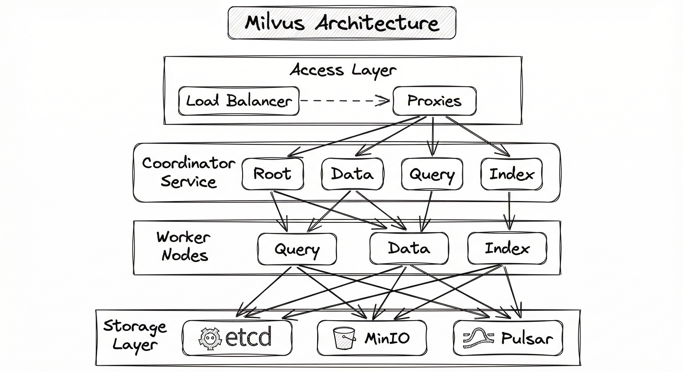
The write path flows through the proxy to data nodes, which write mutations to the log broker (Pulsar/NATS) and periodically flush sealed segments to object storage (MinIO/S3). The read path goes through the proxy to query nodes, which serve queries from a combination of in-memory growing segments (recent data from the log) and sealed segments (historical data loaded from object storage). Index nodes build ANN indices over sealed segments asynchronously.
This separation means you can independently scale query nodes for read-heavy workloads (like a production RAG system serving thousands of requests per second) and data nodes for write-heavy workloads (like a bulk ingestion pipeline processing millions of new embeddings daily).
Key Components
Proxy (Access Layer)
The entry point for all client requests. Proxies are stateless and handle request validation, routing, result aggregation, and rate limiting. They expose gRPC and RESTful APIs. Multiple proxies sit behind a load balancer for high availability.
Root Coordinator
The brain of the cluster. Manages collection metadata (schema, partitions), handles DDL operations (create/drop collection), assigns timestamps for consistency control, and coordinates the other coordinators. Stores metadata in etcd.
Data Coordinator
Manages the lifecycle of data segments. Decides when growing segments should be sealed (based on size or time thresholds), assigns data nodes to log subscriptions, and triggers flush operations to object storage.
Query Coordinator
Manages the distribution of sealed segments across query nodes. Handles load balancing of segments, assigns new segments to query nodes as they are sealed, and manages handoff from data nodes to query nodes.
Index Coordinator
Orchestrates index building. When segments are sealed, the index coordinator assigns index-building tasks to index nodes. Tracks index build progress and manages index metadata.
Query Nodes
The workhorses for search. Each query node loads a subset of sealed segments from object storage into memory (or memory-mapped files) and subscribes to the log broker for growing segments. Executes ANN search and scalar filtering. The core search engine is Knowhere, Milvus's internal vector execution engine that wraps FAISS, HNSWlib, DiskANN, and NVIDIA cuVS.
Data Nodes
Consume mutation logs from the log broker, buffer inserts into growing segments in memory, and flush sealed segments to object storage (MinIO/S3). Also handle delete operations by maintaining a delete log.
Index Nodes
Build ANN indices over sealed segments. Index building is CPU-intensive (or GPU-intensive for GPU indices), so having dedicated index nodes prevents index construction from interfering with query serving.
Knowhere (Vector Engine)
Milvus's internal vector search engine. Knowhere is a C++ library that abstracts over multiple ANN implementations: FAISS (IVF_FLAT, IVF_SQ8, IVF_PQ), HNSWlib (HNSW), DiskANN, NVIDIA cuVS (GPU_CAGRA, GPU_IVF_FLAT, GPU_IVF_PQ). It accounts for over 80% of Milvus's compute resource consumption.
etcd (Metadata Store)
Stores cluster metadata: collection schemas, partition info, segment allocation, node registration, and health checks. etcd's strong consistency guarantees ensure that metadata operations are atomic and durable.
MinIO / S3 (Object Storage)
Persists sealed segments, index files, and binlog data. This is where the bulk of data lives durably. Supports S3, Azure Blob, GCS, or any S3-compatible storage. The use of cheap object storage is what makes Milvus cost-effective at billion scale.
Log Broker (Pulsar / NATS / Kafka)
The backbone of Milvus's streaming architecture. All mutations flow through the log broker, enabling decoupled writes, exactly-once delivery (with Pulsar), and simple node recovery through log replay. Milvus 2.5+ supports NATS as a lightweight alternative to Pulsar for simpler deployments.
Data Flow
- Client sends an insert/upsert/delete request to the Proxy.
- Proxy assigns a timestamp (from Root Coord) and publishes the mutation to the Log Broker (Pulsar/NATS).
- Data Nodes subscribe to the log, buffer mutations into growing segments in memory.
- When a growing segment reaches the configured size threshold (~512 MB by default), Data Coord triggers a seal operation.
- The sealed segment is flushed to Object Storage (MinIO/S3).
- Index Coord detects the new sealed segment and assigns an Index Node to build an ANN index.
- The built index is uploaded to Object Storage.
- Client sends a search request to the Proxy.
- Proxy fans out the query to the relevant Query Nodes (based on which nodes hold the target segments).
- Each Query Node searches both its growing segments (in-memory, unindexed brute-force) and sealed segments (indexed ANN search).
- Results from all Query Nodes are merged at the Proxy, sorted by score, and the top-k are returned to the client.
The write and read paths share no state except through the log broker and object storage, which is why Milvus can scale them independently.
A four-layer architecture diagram showing: (1) Access Layer with load-balanced Proxy nodes at the top, (2) Coordinator Service with Root, Data, Query, and Index Coordinators in the middle, (3) Worker Nodes with Query Nodes, Data Nodes, and Index Nodes below, and (4) Storage Layer at the bottom with etcd for metadata, MinIO/S3 for object storage, and Pulsar/NATS as the log broker. Arrows flow from proxies through coordinators to workers and down to storage.
How to Implement
Three Deployment Modes
Milvus offers three deployment modes, each suited to a different stage of your project:
-
Milvus Lite: An embedded, lightweight version that runs entirely within your Python process. No Docker, no external dependencies. Perfect for prototyping, unit tests, and small datasets (<1M vectors). Just
pip install pymilvusand point the client at a local file. -
Milvus Standalone: A single-node deployment that runs all components in a single Docker container (or docker-compose). Suitable for development, staging, and moderate production workloads (up to ~10M vectors). Requires Docker.
-
Milvus Distributed: The full cluster mode with all components running as separate microservices on Kubernetes. This is what you use for production at scale. Requires a Kubernetes cluster, Helm, etcd, MinIO/S3, and a log broker (Pulsar or NATS).
Zilliz Cloud is the fully managed option -- Milvus-as-a-Service. You get the full distributed architecture without managing any infrastructure. Pricing starts free for prototyping, with dedicated clusters from 4 per million vCUs (virtual compute units).
The Migration Path
Here is why Milvus's multi-mode approach is clever: the same pymilvus code that runs against Milvus Lite on your laptop works identically against Milvus Distributed in production. The only thing that changes is the connection URI. This means you can prototype locally, test against Standalone in CI, and deploy to Distributed (or Zilliz Cloud) in production -- all without changing a single line of application code.
Cost Tip for Indian Startups: Start with Milvus Lite during development (free). Move to Milvus Standalone on a single cloud VM (INR 3,000-5,000/month on AWS ap-south-1 or Azure Central India) for early production. Upgrade to Distributed or Zilliz Cloud only when you need to scale beyond what a single node can handle. This staged approach keeps costs under control while maintaining a clear upgrade path.
from pymilvus import MilvusClient
import numpy as np

# Milvus Lite: just pass a local file path as the URI
client = MilvusClient(uri="./milvus_demo.db")

# Create a collection with auto-generated ID
client.create_collection(
    collection_name="articles",
    dimension=768,
    metric_type="COSINE",
)

# Generate sample embeddings (in production, use your embedding model)
np.random.seed(42)
embeddings = np.random.rand(1000, 768).astype(np.float32)

# Prepare data with metadata
data = [
    {
        "id": i,
        "vector": embeddings[i].tolist(),
        "title": f"Article {i}",
        "category": np.random.choice(["tech", "finance", "health"]),
        "year": int(np.random.choice([2023, 2024, 2025])),
    }
    for i in range(1000)
]

# Insert data
result = client.insert(collection_name="articles", data=data)
print(f"Inserted {result['insert_count']} vectors")

# Search with metadata filter
query_vector = np.random.rand(768).astype(np.float32).tolist()

results = client.search(
    collection_name="articles",
    data=[query_vector],
    filter='category == "tech" and year >= 2024',
    limit=5,
    output_fields=["title", "category", "year"],
)

for hits in results:
    for hit in hits:
        print(f"  ID: {hit['id']}, Score: {hit['distance']:.4f}, "
              f"Title: {hit['entity']['title']}, "
              f"Category: {hit['entity']['category']}")
This example demonstrates Milvus Lite -- the embedded mode that requires zero infrastructure. By passing a local file path as the URI, pymilvus runs Milvus entirely in-process. The same code works with Milvus Standalone or Distributed by simply changing the URI to http://localhost:19530 or your cluster endpoint. Notice how metadata filtering (category == "tech" and year >= 2024) is integrated directly into the search call -- this is Milvus's hybrid scalar+vector query capability.
from pymilvus import (
    connections, Collection, FieldSchema, CollectionSchema,
    DataType, utility
)

# Connect to Milvus Standalone or Distributed
connections.connect(host="localhost", port="19530")

# Define schema
fields = [
    FieldSchema(name="id", dtype=DataType.INT64, is_primary=True, auto_id=True),
    FieldSchema(name="product_embedding", dtype=DataType.FLOAT_VECTOR, dim=768),
    FieldSchema(name="product_name", dtype=DataType.VARCHAR, max_length=256),
    FieldSchema(name="category", dtype=DataType.VARCHAR, max_length=64),
    FieldSchema(name="price_inr", dtype=DataType.FLOAT),
    FieldSchema(name="seller_city", dtype=DataType.VARCHAR, max_length=64),
]

schema = CollectionSchema(
    fields=fields,
    description="Product catalog embeddings for similarity search",
    enable_dynamic_field=True,  # Allow additional fields without schema changes
)

# Create collection with 8 shards for parallel ingestion
collection = Collection(
    name="product_catalog",
    schema=schema,
    num_shards=8,
    consistency_level="Bounded",  # Default: good balance of freshness and performance
)

# Create partitions by product category for faster filtered search
for category in ["electronics", "fashion", "grocery", "home"]:
    collection.create_partition(partition_name=category)

# Build HNSW index for high-recall production search
index_params = {
    "index_type": "HNSW",
    "metric_type": "COSINE",
    "params": {
        "M": 16,            # Number of bi-directional links per node
        "efConstruction": 256,  # Build-time search width (higher = better graph quality)
    },
}
collection.create_index(
    field_name="product_embedding",
    index_params=index_params,
)

# Create scalar index on category for fast filtered search
collection.create_index(
    field_name="category",
    index_name="idx_category",
)

# Load collection into memory
collection.load()

print(f"Collection '{collection.name}' ready.")
print(f"  Entities: {collection.num_entities}")
print(f"  Partitions: {[p.name for p in collection.partitions]}")
This example shows a production-grade collection setup with several important patterns:
- Explicit schema: Define fields with types and constraints rather than relying on auto-detection.
- Sharding: 8 shards enable parallel ingestion across multiple data nodes.
- Partitions by category: Queries that filter by category can skip irrelevant partitions entirely, reducing search scope.
- HNSW index with tuned parameters:
M=16gives a good balance of graph connectivity and memory overhead.efConstruction=256builds a higher-quality graph (at the cost of longer build time). - Scalar index on category: Pre-filtering on indexed scalar fields is much faster than post-filtering.
- Bounded consistency: The default for most production workloads -- allows slightly stale reads but avoids the performance cost of strong consistency.
from pymilvus import connections, Collection, utility

connections.connect(host="localhost", port="19530")

collection = Collection("product_catalog")

# Build GPU_CAGRA index (requires NVIDIA GPU with CUDA support)
gpu_index_params = {
    "index_type": "GPU_CAGRA",
    "metric_type": "L2",
    "params": {
        "intermediate_graph_degree": 128,  # Graph degree during build
        "graph_degree": 64,                # Final graph degree
    },
}

collection.release()  # Release existing index from memory
collection.drop_index()  # Drop old index
collection.create_index(
    field_name="product_embedding",
    index_params=gpu_index_params,
)
collection.load()

# Search with GPU-optimized parameters
search_params = {
    "metric_type": "L2",
    "params": {
        "itopk_size": 128,     # Internal top-k candidates (higher = better recall)
        "search_width": 4,     # Number of entry points in the graph
        "team_size": 0,        # Auto-select based on dimension
    },
}

results = collection.search(
    data=[query_embedding],
    anns_field="product_embedding",
    param=search_params,
    limit=10,
    output_fields=["product_name", "price_inr"],
)

for hits in results:
    for hit in hits:
        print(f"  {hit.entity.get('product_name')}: "
              f"INR {hit.entity.get('price_inr'):.0f} "
              f"(distance: {hit.distance:.4f})")
GPU_CAGRA (CUDA Approximate Nearest Neighbor GRAph) is NVIDIA's graph-based index that leverages GPU parallelism for both index building and search. In benchmarks, CAGRA delivers up to 50x faster search than CPU-based HNSW at equivalent recall. The key parameters are intermediate_graph_degree (higher values build a better graph but take more GPU memory during construction) and graph_degree (the final graph connectivity -- 64 is a good default). Note that GPU_CAGRA requires an NVIDIA GPU with CUDA support -- inference-grade GPUs like T4 or A10G work well and are more cost-effective than training-grade A100s for this workload.
from pymilvus import (
    connections, Collection, AnnSearchRequest,
    WeightedRanker, RRFRanker
)

connections.connect(host="localhost", port="19530")
collection = Collection("hybrid_docs")

# Assume collection has both dense_vector and sparse_vector fields
# with separate indices built on each

# Dense vector search request (semantic)
dense_req = AnnSearchRequest(
    data=[dense_query_embedding],    # From a dense encoder like BGE-M3
    anns_field="dense_vector",
    param={"metric_type": "COSINE", "params": {"ef": 128}},
    limit=20,
)

# Sparse vector search request (lexical/keyword-like)
sparse_req = AnnSearchRequest(
    data=[sparse_query_embedding],   # From BM25 or SPLADE
    anns_field="sparse_vector",
    param={"metric_type": "IP", "params": {}},
    limit=20,
)

# Combine with Reciprocal Rank Fusion (balances both signals)
results = collection.hybrid_search(
    reqs=[dense_req, sparse_req],
    ranker=RRFRanker(k=60),       # RRF with k=60 (standard)
    limit=10,
    output_fields=["title", "chunk_text"],
)

# Alternative: weighted combination
# ranker = WeightedRanker(0.7, 0.3)  # 70% dense, 30% sparse

for hits in results:
    for hit in hits:
        print(f"  Score: {hit.distance:.4f} | {hit.entity.get('title')}")
Milvus 2.5 introduced native hybrid search, letting you combine dense vector search (for semantic similarity) with sparse vector search (for keyword matching) in a single query. This is critical for production RAG systems where pure semantic search misses exact terms (e.g., product codes, Indian pin codes, technical abbreviations). The RRFRanker with is a parameter-free way to fuse rankings from both signals, while WeightedRanker lets you tune the balance manually. In Milvus 2.5+, full-text search with BM25 achieves 3-4x higher throughput than Elasticsearch at equivalent recall.
# docker-compose.yml for Milvus Standalone (development/staging)
version: '3.5'
services:
  etcd:
    image: quay.io/coreos/etcd:v3.5.16
    environment:
      ETCD_AUTO_COMPACTION_MODE: revision
      ETCD_AUTO_COMPACTION_RETENTION: "1000"
      ETCD_QUOTA_BACKEND_BYTES: "4294967296"  # 4 GB
    volumes:
      - etcd_data:/etcd
    command: etcd -advertise-client-urls=http://127.0.0.1:2379 -listen-client-urls http://0.0.0.0:2379

  minio:
    image: minio/minio:RELEASE.2024-09-13T20-26-02Z
    environment:
      MINIO_ACCESS_KEY: minioadmin
      MINIO_SECRET_KEY: minioadmin
    volumes:
      - minio_data:/minio_data
    command: minio server /minio_data

  milvus:
    image: milvusdb/milvus:v2.5.4
    command: ["milvus", "run", "standalone"]
    environment:
      ETCD_ENDPOINTS: etcd:2379
      MINIO_ADDRESS: minio:9000
    ports:
      - "19530:19530"   # gRPC API
      - "9091:9091"     # Metrics (Prometheus)
    volumes:
      - milvus_data:/var/lib/milvus
    depends_on:
      - etcd
      - minio

volumes:
  etcd_data:
  minio_data:
  milvus_data:
Common Implementation Mistakes
- ●
Skipping index creation entirely: New Milvus users often insert data and immediately search without building an index. Milvus will fall back to brute-force search, which works fine for 10K vectors but becomes unusable at 1M+. Always create an index before calling
collection.load(). - ●
Using strong consistency by default: Strong consistency forces every query to wait for all pending writes to be visible. This adds significant latency (often 50-200ms) and is unnecessary for most use cases. Use
Bounded(the default) orSessionconsistency instead. ReserveStrongonly for workflows where a user writes data and immediately needs to search for it in the same request. - ●
Over-provisioning shards: Setting
num_shardsto a large number (e.g., 64) on a small cluster wastes resources. Each shard creates overhead in the coordinator and data nodes. A good rule of thumb: set shards to 2x the number of data nodes for write-heavy workloads, or just use the default (1-2) for read-heavy workloads. - ●
Ignoring partition pruning: If you have a natural partitioning key (like category, region, or tenant_id), use Milvus partitions. Searching within a specific partition skips all other partitions entirely, which can reduce search latency by 5-10x for selective queries. But avoid creating more than 1,024 partitions per collection -- beyond that, metadata overhead dominates.
- ●
Loading entire collections into memory when only a subset is needed: If you only query certain partitions, load just those partitions with
collection.load(partition_names=["electronics"]). Loading the full collection wastes memory on data you never search. - ●
Mixing vectors from different embedding models in the same collection: Just like with any vector store, vectors from different models live in incompatible geometric spaces. If you upgrade your embedding model, you must re-embed and re-index. Use blue-green deployment: build a new collection with the updated model, validate, then swap.
- ●
Not setting
efConstructionhigh enough during HNSW index build: The defaultefConstruction=128is adequate for small datasets, but for 10M+ vectors, increasing it to 256 or 512 produces a significantly better graph. This is a one-time cost at build time that pays dividends on every query.
When Should You Use This?
Use When
You need to serve similarity search at billion scale (100M+ vectors) with sub-100ms latency and your team has the engineering capacity to operate a distributed system
Your workload requires independent scaling of reads and writes -- for example, a recommendation engine with bursty read traffic and steady background ingestion
You need GPU-accelerated vector search to maximize throughput on existing GPU infrastructure (e.g., you already have NVIDIA T4s or A10Gs for inference)
Your application requires tunable consistency levels -- strong consistency for real-time collaborative workflows, bounded staleness for analytics, eventual consistency for batch recommendation pipelines
You are building a multi-tenant RAG system that needs partition-based isolation and per-tenant metadata filtering at scale
You want an open-source solution with no vendor lock-in and the ability to self-host on your own infrastructure (important for Indian enterprises with data residency requirements)
Your pipeline needs hybrid search combining dense vector similarity with sparse/BM25 keyword matching in a single query
You need support for multiple index types and want to experiment with different recall-throughput-memory tradeoffs (IVF_FLAT for prototyping, HNSW for production, DiskANN for cost-sensitive deployments)
Avoid When
Your dataset is small (<500K vectors) and a simpler solution like Qdrant (single binary, minimal ops), pgvector (if you are already on PostgreSQL), or Chroma (for prototyping) would be sufficient
You want a fully managed, zero-ops experience and are willing to pay a premium -- Pinecone is simpler to operate than self-hosted Milvus, and Zilliz Cloud is a managed Milvus but still requires understanding Milvus concepts
Your team lacks Kubernetes expertise -- Milvus Distributed requires a Kubernetes cluster, Helm charts, and familiarity with etcd/MinIO/Pulsar. The operational complexity is non-trivial
You need strong ACID transactions across vector and scalar data -- Milvus is not a general-purpose transactional database. If you need joins, foreign keys, and transactions alongside vector search, consider pgvector
Your primary bottleneck is filtering on scalar attributes rather than vector similarity -- a traditional database with standard indices will be simpler and possibly faster for this use case
You are building a quick prototype or hackathon project where Milvus Lite or Chroma would get you to a working demo in minutes without any infrastructure overhead
Key Tradeoffs
The Power-Complexity Tradeoff
Milvus is the most feature-rich open-source vector database available today. It is also the most operationally complex. Running Milvus Distributed requires etcd (for metadata), MinIO or S3 (for object storage), a log broker (Pulsar, NATS, or Kafka), and multiple microservices (proxies, coordinators, workers) -- all orchestrated on Kubernetes.
This complexity is the price you pay for true horizontal scalability. If you need to serve 50,000 QPS over 1 billion vectors with independent scaling of reads and writes, Milvus is one of the few open-source options that can do it. But if you are serving 500 QPS over 5 million vectors, you are over-engineering.
| Factor | Milvus | Qdrant | Pinecone | pgvector |
|---|---|---|---|---|
| Max proven scale | Billions | 100M+ | Billions | ~10M |
| Operational complexity | High | Medium | Low (managed) | Low (PostgreSQL) |
| GPU support | Yes (CAGRA) | No | No | No |
| Hybrid search | Native (2.5+) | Basic | Yes | Limited |
| Self-hosted cost (10M vectors) | ~$200/mo (~INR 16,800) | ~$100/mo (~INR 8,400) | ~$70-300/mo (~INR 5,900-25,200) | ~$50/mo (~INR 4,200) |
| Managed cost (10M vectors) | Zilliz ~$99/mo | Qdrant Cloud ~$65/mo | ~$70/mo | Neon/Supabase ~$25/mo |
Memory vs. Disk: The Index Type Decision
With Milvus, you have fine-grained control over where your index lives:
- In-memory (HNSW): Fastest queries (1-5ms), but costs scale linearly with data size. For 100M x 768-dim vectors: ~400 GB RAM = ~$3,200/mo (~INR 2.7 lakh/mo) on AWS.
- In-memory compressed (IVF_SQ8): 75% less memory than HNSW with ~1-2% recall loss. Same 100M vectors: ~100 GB RAM = ~$800/mo (~INR 67,000/mo).
- On-disk (DiskANN): Index lives on SSD, only metadata in memory. Same 100M vectors: ~50 GB SSD + 10 GB RAM = ~$200/mo (~INR 16,800/mo). But query latency rises to 5-20ms.
- GPU (CAGRA): Fastest build and query times, but requires GPU instances. An NVIDIA T4 instance on AWS Mumbai region costs ~$280/mo (~INR 23,500/mo) and can handle 50-100M vectors.
Decision Rule: Start with HNSW if you can afford the memory. Move to IVF_SQ8 or DiskANN when costs exceed your budget. Use GPU_CAGRA when throughput requirements are extreme and you already have GPU infrastructure.
Alternatives & Comparisons
Pinecone is a fully managed vector database -- zero ops, no infrastructure to maintain. Choose Pinecone when your team wants to focus entirely on the application layer and is willing to pay a premium for operational simplicity. Choose Milvus when you need the control and cost advantages of self-hosting, require GPU acceleration, or need to keep data on-premises (common for Indian banking and government projects with data residency requirements).
Qdrant is an excellent choice for teams that want strong vector search performance with lower operational complexity than Milvus. Written in Rust, it is fast, memory-efficient, and easy to deploy as a single binary. Choose Qdrant for workloads up to ~100M vectors where simplicity matters. Choose Milvus when you need true billion-scale distributed search, GPU acceleration, or the broadest selection of index types.
Weaviate provides built-in vectorization modules and a GraphQL API, making it appealing for teams that want embedding generation integrated into the database layer. Choose Weaviate when you want a more opinionated, batteries-included experience with GraphQL. Choose Milvus when you want maximum control over indexing, need GPU support, or are working at scales beyond what Weaviate's architecture supports efficiently.
Chroma is the simplest way to get started with vector search -- pip install chromadb and you are running. It is perfect for prototyping, small datasets, and educational projects. Choose Chroma when speed of development matters more than production scale. Choose Milvus when you need to go beyond a single node, require advanced features like GPU indexing or tunable consistency, or are building for production scale.
pgvector adds vector search to PostgreSQL, letting you keep vector data alongside relational data in a single database. Choose pgvector when you are already running PostgreSQL, your vector corpus is under ~10M, and you want to avoid introducing a separate system. Choose Milvus when you need dedicated vector search performance at scale, GPU acceleration, or advanced ANN index types beyond what pgvector's IVF and HNSW support provides.
Pros, Cons & Tradeoffs
Advantages
Proven at billion scale: Milvus is one of the few open-source vector databases with production deployments at 1B+ vectors. NVIDIA runs it over tens of billions of vectorized sensor data points for autonomous driving. This is not theoretical -- it is battle-tested.
Broadest index type support: IVF_FLAT, IVF_SQ8, IVF_PQ, HNSW, SCANN, DiskANN, GPU_IVF_FLAT, GPU_IVF_PQ, GPU_CAGRA, and FLAT. No other vector database gives you this many options to tune the recall-throughput-memory tradeoff for your specific workload.
GPU acceleration via NVIDIA CAGRA: Up to 50x faster search compared to CPU-based HNSW. This is a genuine differentiator -- no other open-source vector database offers GPU-accelerated indexing and search at this level of maturity.
True disaggregated architecture: Storage and compute scale independently. You can add query nodes for read traffic without touching data nodes, and vice versa. This makes capacity planning much more predictable than monolithic alternatives.
Native hybrid search (Milvus 2.5+): Combine dense vector similarity with sparse vector / BM25 full-text search in a single query. Benchmarks show 3-4x higher throughput than Elasticsearch at equivalent recall.
Tunable consistency levels: Strong, Bounded, Session, and Eventually -- the same consistency spectrum as DynamoDB or Cassandra, but for vector search. This is rare in the vector database world.
Smooth migration path: Milvus Lite (embedded) -> Standalone (Docker) -> Distributed (Kubernetes) -> Zilliz Cloud (managed). Same API, same code, different scale.
Strong open-source community: 40K+ GitHub stars, LF AI & Data Foundation project, active Discord, and a SIGMOD paper. This is a project with institutional backing, not a weekend side project.
Disadvantages
High operational complexity for distributed mode: Running Milvus Distributed requires etcd, MinIO/S3, a log broker (Pulsar/NATS/Kafka), and Kubernetes. The dependency chain is long, and each component needs monitoring and maintenance. For a team of 2-3 engineers at an Indian startup, this can be overwhelming.
Resource-hungry dependencies: etcd requires low-latency disks, Pulsar is itself a distributed system that needs ZooKeeper (unless using NATS). The total memory footprint of the control plane can exceed 8-12 GB before you even load any vectors.
Steeper learning curve than alternatives: Concepts like segments, sealed vs. growing, consistency levels, partition keys, and shard management are powerful but add cognitive overhead. Qdrant and Pinecone are simpler to reason about for common use cases.
Cold start latency: When query nodes load sealed segments from object storage, there can be significant startup delay (minutes for large collections). This affects scaling responsiveness and recovery time after crashes.
Metadata filtering performance with post-filtering: While Milvus supports pre-filtering for indexed scalar fields, complex filter expressions on non-indexed fields fall back to post-filtering, which can return fewer than k results for selective predicates.
Limited ecosystem outside Python: While
pymilvusis mature, SDKs for Java, Go, and Node.js are less feature-complete. Most documentation and examples are Python-first.Version upgrade complexity: Upgrading between major versions (e.g., 2.4 to 2.5) can require careful planning due to changes in metadata schema, index format, and dependency versions. The migration guides exist but are non-trivial.
Failure Modes & Debugging
etcd Metadata Corruption or Exhaustion
Cause
etcd runs out of disk space, or the metadata store exceeds its configured quota (ETCD_QUOTA_BACKEND_BYTES). This can happen with frequent DDL operations (create/drop collections) or excessive partition creation.
Symptoms
All DDL operations fail with "etcdserver: mvcc: database space exceeded" errors. New collections cannot be created, and existing collections may become read-only. The cluster appears healthy from the worker node perspective but the coordinator service is effectively frozen.
Mitigation
Set ETCD_QUOTA_BACKEND_BYTES to at least 4 GB (default is 2 GB). Enable auto-compaction with ETCD_AUTO_COMPACTION_MODE=revision and ETCD_AUTO_COMPACTION_RETENTION=1000. Monitor etcd disk usage with Prometheus alerts. Keep the number of collections and partitions reasonable (a few hundred, not tens of thousands).
Query Node OOM During Segment Loading
Cause
Query nodes attempt to load more sealed segments into memory than available RAM. This typically happens when a collection grows beyond initial capacity estimates, or when multiple collections are loaded simultaneously on the same node.
Symptoms
Query nodes crash with OOM kills (exit code 137 on Kubernetes). Pods enter CrashLoopBackOff. Queries timeout or return errors. The Query Coordinator repeatedly assigns the same segments to the restarting node, creating a crash loop.
Mitigation
Use mmap for large collections: Milvus supports memory-mapped segment loading, which uses disk as backing storage and only pages in data on demand. Enable with queryNode.mmap.enabled=true. Alternatively, use compressed index types (IVF_SQ8, RaBitQ) to reduce per-vector memory. Monitor query node RSS with Prometheus and set Kubernetes resource limits with adequate headroom (1.5x estimated segment size).
Log Broker (Pulsar) Backlog Overflow
Cause
Data ingestion rate exceeds the rate at which data nodes and query nodes consume from the log broker. Pulsar topics accumulate unbounded backlog, consuming disk space and increasing end-to-end write latency.
Symptoms
Insert latency increases progressively. Pulsar disk usage grows rapidly. Data nodes lag behind, causing query nodes to miss recent data (staleness increases beyond Bounded consistency guarantees). In extreme cases, Pulsar brokers OOM.
Mitigation
Monitor Pulsar topic backlog with Pulsar Manager or Prometheus metrics. Scale data nodes to match ingestion throughput. Configure topic retention policies to cap maximum backlog. For simpler deployments, consider switching to NATS (supported in Milvus 2.5+), which has a smaller footprint and simpler operations than Pulsar.
Silent Recall Degradation from Incorrect Metric Type
Cause
The index is built with a distance metric (e.g., L2) that does not match the embedding model's training objective (e.g., cosine similarity). Milvus will build the index and return results -- they will just be geometrically wrong.
Symptoms
Search results are semantically poor. Downstream RAG quality drops. A/B tests show the retrieval pipeline performing near-randomly. No errors or warnings are raised because the query is technically valid.
Mitigation
Always check the embedding model's documentation for the recommended distance metric. For most modern sentence transformers (BGE, E5, GTE), use COSINE. For models trained with Maximum Inner Product Search (MIPS) objectives, use IP. Add a validation step in your CI pipeline that checks metric configuration against model metadata.
Partition Explosion Causing Coordinator Overhead
Cause
Creating too many partitions (thousands) or too many collections (hundreds) in a single Milvus cluster. Each partition and collection adds metadata overhead in etcd and the coordinator service.
Symptoms
DDL operations become slow (seconds to minutes for create/drop). Coordinator startup time increases. etcd latency spikes. In extreme cases (>10,000 partitions across all collections), the cluster becomes unstable.
Mitigation
Use partition keys (introduced in Milvus 2.3) instead of manually creating one partition per tenant. Partition keys let Milvus automatically distribute data across a fixed number of internal partitions based on a hash of the key field. Aim for fewer than 1,024 partitions per collection and fewer than 100 collections per cluster.
Index Build Starvation Under Continuous Ingestion
Cause
New segments are sealed faster than index nodes can build indices. This happens during high-throughput bulk ingestion when index node capacity is insufficient.
Symptoms
Newly ingested data is searchable but uses brute-force scan (no ANN index) on growing segments, causing query latency to spike. The indexing_queue_length metric grows unbounded. Index Coordinator logs show a backlog of pending index tasks.
Mitigation
Scale index nodes during bulk ingestion. Consider using GPU index nodes for faster builds. Temporarily increase the segment seal threshold (dataCoord.segment.maxSize) to create fewer, larger segments. After bulk ingestion completes, reduce the threshold and let the system catch up.
Placement in an ML System
Where Milvus Fits in the ML Pipeline
In a RAG (Retrieval-Augmented Generation) pipeline, Milvus sits after the embedding model has encoded documents/chunks into vectors and before the re-ranker or context assembler that prepares retrieved passages for the LLM. The typical flow is:
- Documents are chunked and embedded offline (or in a streaming pipeline)
- Embeddings are ingested into Milvus with metadata (source, timestamp, tenant_id)
- At query time, the user's question is embedded by the same model
- Milvus returns the top-k most similar chunks, optionally filtered by metadata
- A re-ranker (like a cross-encoder) refines the ranking
- The top passages are assembled into the LLM's context window
In a recommendation system (like Shopee's video recommendation engine), Milvus stores item embeddings and serves as the candidate retrieval layer. User/query embeddings are searched against the item collection to generate a candidate set, which is then scored and ranked by a downstream model.
In an autonomous driving pipeline (like NVIDIA's sensor data platform), Milvus indexes billions of vectorized sensor frames, enabling engineers to run semantic queries like "find me all frames containing a pedestrian crossing in rain" across massive datasets.
For an Indian e-commerce platform, Milvus could power both visual similarity search ("find products that look like this photo") and semantic product search ("comfortable cotton kurta for summer wedding") by indexing image and text embeddings respectively, filtered by category, seller city, and price range.
Pipeline Stage
Retrieval / Serving
Upstream
- embedding-model
- vector-store
- semantic-search
Downstream
- semantic-search
- vector-store
Scaling Bottlenecks
The primary bottlenecks in a Milvus deployment are:
-
Query Node Memory: In-memory indices (HNSW, IVF_FLAT) scale linearly with data size. For 1B vectors at 768 dimensions, you need ~3 TB of RAM for HNSW -- that is a fleet of memory-optimized instances costing $20,000+/month (~INR 16.8 lakh/month). DiskANN and mmap mitigate this but add latency.
-
Log Broker Throughput: The log broker (Pulsar/NATS) is the single funnel for all writes. At very high ingestion rates (>100K inserts/second), the log broker can become the bottleneck. Scaling Pulsar itself is non-trivial.
-
Index Build Throughput: Building HNSW indices over large segments is CPU-intensive. For 100M vectors, expect 2-4 hours of index build time on a 16-core machine. GPU indices (CAGRA) reduce this dramatically but require GPU infrastructure.
-
Cross-Shard Query Latency: When a search spans multiple shards on different query nodes, the proxy must wait for all nodes to respond and merge results. This adds 2-10ms of network overhead per shard, which can add up for highly sharded collections.
-
etcd Metadata Operations: etcd is the bottleneck for DDL operations (create/drop collection, create partition). Keep DDL operations infrequent in production.
Production Case Studies
NVIDIA adopted Milvus to power large-scale multimodal data search for its autonomous driving platform. Engineers run semantic queries over tens of billions of vectorized sensor data points (camera frames, LiDAR scans, radar signals). By replacing FAISS with Milvus, the AV data platform gained distributed scalability, operational reliability, and efficient indexing for mining rare driving scenarios and validating real-world model behavior.
Enabled semantic search over tens of billions of sensor vectors with sub-second query latency. Improved the efficiency of rare-scenario mining for AV model validation, accelerating the development cycle for autonomous driving systems.
Shopee, the leading e-commerce platform in Southeast Asia (with significant presence in India via partnerships), uses Milvus for real-time video recall, copyright matching, and video deduplication. When a user searches for a video, Milvus retrieves the most similar top-K candidates from billions of video embeddings, which are then refined through post-ranking algorithms. Milvus's cloud-native architecture integrated seamlessly with Shopee's internal ecosystem.
Enabled real-time video similarity search over billions of embeddings. Reduced copyright-infringing content through automated deduplication. Shopee is running Milvus in production and plans to upgrade to leverage GPU indexing and range search features.
Salesforce's platform team uses Milvus to support a wide range of internal AI use cases, serving 100+ tenants with diverse applications and varying service levels. Milvus's partition-based isolation and metadata filtering enable multi-tenant vector search at enterprise scale, powering features like semantic document search, AI-assisted customer support, and intelligent lead scoring across Salesforce's vast ecosystem.
Supports 100+ internal tenants with varied AI workloads on a shared Milvus infrastructure. Leverages Milvus's multi-tenancy features for cost-effective, isolated vector search across the Salesforce platform.
Rakuten Symphony (part of the Rakuten Group, which also operates in India through Rakuten India) selected Milvus as their platform of choice for LLM-powered applications. Engineers use Milvus for semantic search and retrieval across their diverse product catalog, financial services documentation, and customer support knowledge bases.
Standardized on Milvus as the vector database platform for all LLM-related use cases across Rakuten Symphony's engineering organization.
Tooling & Ecosystem
The core open-source vector database. Cloud-native, distributed, supports 10+ index types including GPU-accelerated CAGRA. Written in Go and C++. Deployed via Docker or Kubernetes.
The official Python SDK for Milvus. Provides both the high-level MilvusClient API (simple, Pythonic) and the lower-level ORM API (more control). Includes Milvus Lite for embedded usage and integration utilities for embedding models (OpenAI, Sentence Transformers, BGE-M3, SPLADE).
The official web-based GUI for Milvus. Provides visual collection management, schema design, vector search with filters, knowledge graph visualization of search results, system monitoring, and a REST API playground. Think of it as the "pgAdmin for Milvus." Version 2.6.0+ includes a built-in AI assistant and text embedding functions.
Fully managed Milvus-as-a-Service by Zilliz, the company behind Milvus. Available on AWS, Azure, and GCP. Offers serverless (pay-per-query) and dedicated (fixed clusters) tiers. Storage at $0.04/GB/month (standardized across clouds since January 2026). Free tier available for prototyping.
Open-source benchmarking tool for vector databases. Tests real-world scenarios including streaming ingestion, metadata filtering with varying selectivity, and concurrent workloads. Evaluates throughput, latency, recall, and resource utilization across Milvus, Pinecone, Qdrant, Elasticsearch, and others.
Lightweight, embedded version of Milvus that runs entirely within a Python process. No Docker, no external dependencies. Data persists to a local file. Ideal for prototyping, unit testing, and edge deployments. Same API as full Milvus -- migration is just a URI change.
Official backup and restore tool for Milvus. Supports full and incremental backups of collections, including vectors, metadata, and index configurations. Critical for disaster recovery in production deployments.
Research & References
Wang, Yi, Guo, Jin, Xu, Li, Wang, Guo, Li, Xu, Yu, Yuan, et al. (2021)ACM SIGMOD 2021
The foundational paper for Milvus, published at SIGMOD -- one of the top database conferences. Presents Milvus as a cloud-native vector database with heterogeneous computing support, hybrid scalar+vector queries, and a disaggregated storage/compute architecture.
Malkov & Yashunin (2018)IEEE TPAMI, Vol. 42, No. 4
The paper that introduced HNSW -- the multi-layer proximity graph that is now the default index type in Milvus and most other vector databases. Achieves logarithmic search complexity with excellent recall.
Johnson, Douze & Jegou (2021)IEEE Transactions on Big Data
Describes GPU-optimized k-selection and brute-force/IVF search implementations forming the algorithmic basis of FAISS, which underpins Milvus's Knowhere vector engine for IVF-family indices.
Subramanya, Devvrit, Simhadri, Krishnawamy & Kadekodi (2019)NeurIPS 2019
Introduces DiskANN, a graph-based index that stores the graph on SSD while keeping only compressed vectors in memory. Milvus supports DiskANN for cost-effective billion-scale search where memory budget is limited.
Pan, Wang & Li (2024)The VLDB Journal
Comprehensive survey of 20+ vector database systems analyzing indexing, storage, and query processing techniques. Provides detailed comparisons of Milvus against Pinecone, Qdrant, Weaviate, and others across architectural and performance dimensions.
Jegou, Douze & Schmid (2011)IEEE TPAMI, Vol. 33, No. 1
Introduced product quantization (PQ) for decomposing high-dimensional vectors into sub-vector quantization codes. PQ forms the basis of Milvus's IVF_PQ index type, which achieves dramatic memory savings at the cost of some recall.
Interview & Evaluation Perspective
Common Interview Questions
- ●
How does Milvus's architecture differ from a single-node vector database like Qdrant? What are the tradeoffs?
- ●
Explain the four consistency levels in Milvus. When would you choose Bounded over Strong?
- ●
You need to serve 10,000 QPS over 500M product embeddings with sub-50ms P99 latency. Walk me through how you would design this with Milvus.
- ●
What is the difference between IVF_FLAT, IVF_SQ8, and HNSW in Milvus? How do you choose?
- ●
How would you handle a model upgrade (new embedding model) for a Milvus collection with 1B vectors in production?
- ●
Explain how partitions and partition keys work in Milvus. When would you use them?
- ●
How does GPU_CAGRA differ from CPU-based HNSW? When is GPU acceleration worth the cost?
Key Points to Mention
- ●
Milvus disaggregates storage (MinIO/S3) and compute (query/data/index nodes), enabling independent scaling of reads and writes. This is a fundamental architectural advantage over monolithic vector databases.
- ●
The four consistency levels (Strong, Bounded, Session, Eventually) map to different
GuaranteeTsvalues on the internal timestamp oracle. Bounded is the default and right for 90% of production workloads. - ●
Knowhere is the internal vector engine that abstracts over FAISS, HNSWlib, DiskANN, and NVIDIA cuVS. This is why Milvus supports more index types than any other vector database.
- ●
GPU_CAGRA achieves up to 50x faster search than CPU HNSW by leveraging GPU parallelism for graph traversal. But the real win is index build time -- CAGRA builds indices 10-100x faster than HNSW.
- ●
For multi-tenant systems, use partition keys (Milvus 2.3+) instead of one-partition-per-tenant. Partition keys hash data into a fixed number of internal partitions, avoiding the metadata overhead of thousands of explicit partitions.
- ●
Blue-green re-indexing for model upgrades: create a new collection with the updated embedding model, backfill vectors, validate recall against a golden set, swap the alias, then drop the old collection. Never mix vectors from different models.
Pitfalls to Avoid
- ●
Claiming Milvus is 'just a FAISS wrapper' -- Milvus 2.x is a full distributed database with its own WAL, metadata service, query planning, and consistency model. FAISS is one of many index backends accessed through Knowhere.
- ●
Forgetting to mention the operational complexity of Milvus Distributed -- an interviewer will want to hear that you understand the etcd/MinIO/Pulsar dependency chain, not just the API surface.
- ●
Recommending Milvus for every vector search use case regardless of scale. For <5M vectors with simple requirements, Qdrant or pgvector are usually better choices. Show judgment, not fanboyism.
- ●
Ignoring memory planning. A senior candidate should be able to estimate memory requirements: vectors x dimensions x 4 bytes x 1.3 (HNSW overhead) = approximate RAM needed. For 100M x 768-dim vectors: ~400 GB.
- ●
Not knowing about Milvus Lite -- it shows you have not actually used Milvus recently if you think it always requires a Kubernetes cluster.
Senior-Level Expectation
A senior or staff-level candidate should be able to design a complete Milvus deployment from scratch: collection schema with appropriate field types, index type selection with quantitative justification (not just 'I would use HNSW' but 'HNSW with M=16, efConstruction=256 because our recall requirement is 0.97 at k=10 and we have budget for ~400GB RAM'), partition strategy, consistency level choice, capacity planning with cost estimates in both USD and INR, monitoring setup (Prometheus + Grafana with alerts on query latency P99, recall regression, and segment loading time), disaster recovery (Milvus Backup + cross-region replication on Zilliz Cloud), and a re-indexing strategy for embedding model upgrades. The ability to reason about the etcd/Pulsar/MinIO dependency chain and its failure modes separates senior engineers from those who have only used Milvus through LangChain tutorials.
Summary
Wrapping Up
Milvus is the most feature-rich and battle-tested open-source vector database available today. Its disaggregated, cloud-native architecture -- with separate storage (MinIO/S3), compute (query/data/index nodes), metadata (etcd), and streaming (Pulsar/NATS) layers -- enables true horizontal scaling for billion-vector workloads. With support for 10+ index types (including GPU-accelerated CAGRA), four tunable consistency levels, native hybrid search, and a smooth Lite-to-Distributed migration path, Milvus gives ML engineers unprecedented control over the recall-throughput-memory-cost tradeoff.
But that power comes with complexity. Running Milvus Distributed is not a weekend project -- it requires Kubernetes expertise, understanding of the etcd/Pulsar dependency chain, and careful capacity planning. For small-to-medium workloads (<10M vectors), simpler alternatives like Qdrant, pgvector, or even Milvus Lite may serve you better. The right choice depends on your scale, your team's operational maturity, and your budget constraints.
For Indian ML teams specifically, Milvus offers a compelling combination: open-source (no licensing costs), self-hostable (data residency compliance for BFSI and government projects), and deployable on Indian cloud regions (AWS Mumbai, Azure Central India). Start with Milvus Lite for prototyping at zero cost, move to Standalone on a single VM for early production (~INR 10,000-15,000/month), and scale to Distributed or Zilliz Cloud only when your data and traffic demand it. The pymilvus API stays the same throughout -- your code grows with your scale, not against it.