Explainer (SHAP) in Machine Learning
SHAP (SHapley Additive exPlanations) is a unified framework for interpreting the predictions of any machine learning model by assigning each input feature a contribution value grounded in cooperative game theory. It answers the question every stakeholder -- from the data scientist debugging a fraud model to the RBI auditor reviewing a credit scoring system -- eventually asks: why did the model make this particular prediction?
SHAP bridges the gap between high-accuracy black-box models (gradient-boosted trees, deep neural networks, ensemble stacks) and the transparency requirements of regulated industries. By rooting feature attributions in Shapley values -- a concept from economics with over 70 years of axiomatic justification -- SHAP provides explanations that are mathematically consistent, locally accurate, and additive across features.
In the Indian context, where the Reserve Bank of India increasingly demands algorithmic transparency for lending and insurance models, and globally under the EU AI Act's high-risk system requirements, SHAP has become the de facto standard for post-hoc model explanations. Whether you are building a loan approval model at Razorpay, a risk scoring engine at CRED, or a medical diagnosis system at Practo, understanding SHAP is no longer optional -- it is a regulatory and ethical necessity.
This guide covers everything from the mathematical foundations of Shapley values to production-grade deployment patterns, GPU acceleration, and the nuances of choosing between TreeSHAP, DeepSHAP, and KernelSHAP for your specific model architecture.
Concept Snapshot
- What It Is
- A game-theoretic framework that assigns each input feature a contribution (Shapley value) to a specific model prediction, providing both local and global model interpretability.
- Category
- Responsible AI
- Complexity
- Intermediate
- Inputs / Outputs
- Inputs: a trained ML model + a single data instance (or batch). Outputs: per-feature attribution values (SHAP values) that sum to the difference between the model's prediction and the expected prediction.
- System Placement
- Sits as a post-hoc explanation layer after model training and inference, consuming model predictions and producing human-readable feature attributions for monitoring, auditing, and debugging.
- Also Known As
- Shapley Additive Explanations, SHAP values, Shapley feature attributions, SHAP explainer, model-agnostic explanations
- Typical Users
- ML Engineers, Data Scientists, Model Risk Analysts, Compliance Officers, Product Managers, Regulatory Auditors
- Prerequisites
- Basic probability and statistics, Understanding of ML model types (trees, neural networks), Feature engineering concepts, Familiarity with model evaluation metrics
- Key Terms
- Shapley valuecooperative game theorymarginal contributioncoalitionTreeSHAPKernelSHAPDeepSHAPbase valuefeature attributionadditivity
Why This Concept Exists
The Black-Box Problem
Modern ML systems achieve remarkable accuracy -- XGBoost winning Kaggle competitions, deep transformers crushing NLP benchmarks, ensemble stacks powering credit decisions at scale. But accuracy alone is not enough. When a model denies a loan to a farmer in rural Maharashtra, or flags a legitimate UPI transaction as fraudulent on PhonePe, someone needs to explain why.
Traditional feature importance methods (permutation importance, Gini importance, correlation analysis) provide only global explanations: "income is the most important feature overall." They cannot tell you why this specific applicant was rejected. SHAP fills that gap by providing local, instance-level explanations that are mathematically grounded.
The Fragmented Landscape Before SHAP
Before Lundberg and Lee's 2017 NeurIPS paper, the interpretability landscape was fragmented. LIME offered local linear approximations. DeepLIFT explained neural networks by comparing activations to a reference. Integrated Gradients accumulated gradients along a path. Layer-wise Relevance Propagation (LRP) backpropagated relevance scores. Each method had its own assumptions, properties, and failure modes.
The breakthrough insight of SHAP was recognizing that all these methods are special cases of a single framework rooted in Shapley values. By unifying them under one theoretical umbrella, SHAP provided:
- Consistency: If a model changes so that a feature's contribution increases, its SHAP value never decreases.
- Local accuracy: SHAP values for a prediction sum exactly to the difference between the predicted value and the base (expected) value.
- Missingness: Features that are absent (missing) are assigned a SHAP value of zero.
No prior method simultaneously guaranteed all three properties.
Regulatory Tailwinds
The regulatory environment has accelerated SHAP adoption dramatically:
- EU AI Act (2025): High-risk AI systems (including credit scoring, hiring, and insurance) must provide transparent explanations of their decisions. Article 13 explicitly requires that deployers can interpret system outputs. SHAP is the most widely adopted technique for meeting these requirements.
- RBI Guidelines (India): The Reserve Bank of India's evolving digital lending guidelines require lenders to disclose the logic behind algorithmic credit decisions. While the RBI hasn't mandated a specific XAI technique, SHAP's additive decomposition maps directly to the "key factors affecting the credit decision" that must be communicated to borrowers under the 2022 Digital Lending Guidelines.
- US SR 11-7 (OCC/Fed): Model risk management guidance in the US banking sector requires that models be interpretable and validated -- SHAP is the tool of choice for model validation teams at institutions like JPMorgan, Goldman Sachs, and ICICI Bank.
Key Takeaway: SHAP exists because we needed a mathematically rigorous, unified framework for model explanation that satisfies both the technical requirements of ML engineers and the transparency demands of regulators and end-users.
Core Intuition & Mental Model
The Pizza Analogy
Imagine four friends order a pizza together. The total bill is INR 800. How should they split it fairly? One person chose the expensive toppings, another selected the restaurant, a third negotiated a discount, and the fourth just showed up. The Shapley value from game theory provides the unique fair allocation: it considers every possible ordering in which the friends could have joined the group and averages each person's marginal contribution across all orderings.
SHAP does exactly the same thing, but for features in a model prediction. The "total bill" is the model's prediction for a specific input. The "friends" are the input features. SHAP computes the average marginal contribution of each feature across all possible coalitions (subsets) of features.
From Global to Local
Here is the critical mental shift: traditional feature importance tells you which features matter on average across all predictions. SHAP tells you which features matter for this specific prediction. This is the difference between "income is generally important for loan decisions" and "for this applicant, their high debt-to-income ratio pushed the prediction from 'approve' to 'reject' by 0.23."
The beauty of SHAP is that you get both: aggregate the local SHAP values across many predictions, and you recover global feature importance. But you can always drill down to a single prediction and explain exactly what happened. It is like having a microscope and a telescope in one instrument.
The Base Value Anchor
Every SHAP explanation starts from a base value -- the model's average prediction across the training data (or a background dataset). For a binary classifier, this might be 0.35 (the average probability of the positive class). Each feature's SHAP value then pushes the prediction up or down from this base value. The sum of all SHAP values plus the base value equals the model's actual prediction for that instance. No approximation, no residual -- exact decomposition.
This additive property is what makes SHAP explanations so intuitive: you can literally walk through a prediction as a sequence of pushes and pulls, feature by feature, starting from the average and arriving at the final prediction. The waterfall plot visualizes exactly this journey.
Technical Foundations
Shapley Values: The Mathematical Foundation
Let be a trained model and be an input instance with features. The Shapley value for feature is defined as:
where:
- is the set of all features
- is a subset (coalition) of features not containing
- is the model's expected output when only features in are "present" and the remaining features are marginalized out
- The weighting factor counts the fraction of permutations where precedes
The SHAP Axioms
Shapley values are the unique set of feature attributions satisfying these four axioms simultaneously:
-
Efficiency (Local Accuracy): where is the base value. The attributions fully decompose the prediction.
-
Symmetry: If features and contribute equally in all coalitions, then .
-
Dummy (Missingness): If feature does not change the output in any coalition, then .
-
Additivity: For an additive model , the Shapley values decompose: . This is why SHAP works naturally for ensembles.
Computational Complexity
The exact Shapley value formula requires summing over all subsets of features for each feature . The total computation is model evaluations. For a model with 50 features, that is evaluations -- completely infeasible.
This exponential complexity is why approximation algorithms are essential:
| Algorithm | Complexity | Model Type | Exact? |
|---|---|---|---|
| KernelSHAP | where = samples | Any (model-agnostic) | No (sampling-based) |
| TreeSHAP | Tree ensembles | Yes | |
| DeepSHAP | Neural networks | No (approximation) | |
| LinearSHAP | Linear models | Yes | |
| Exact | Any | Yes |
where = number of trees, = max leaves, = max depth.
The SHAP Kernel
KernelSHAP formulates the Shapley value computation as a weighted linear regression problem. It assigns a weight to each coalition :
Coalitions near the extremes (very few or very many features present) receive the highest weights, which is intuitive: including or excluding a single feature tells you more about its marginal effect than halfway coalitions.
Mathematical Insight: The Shapley value is not just a way to distribute credit among features -- it is the only way that satisfies all four axioms simultaneously. This uniqueness theorem (proved by Shapley in 1953) is what gives SHAP its theoretical authority over ad-hoc feature importance methods.
Internal Architecture
The SHAP explanation pipeline consists of four primary stages: model wrapping, background data selection, Shapley value computation, and visualization/reporting. The choice of explainer algorithm depends on the model type.
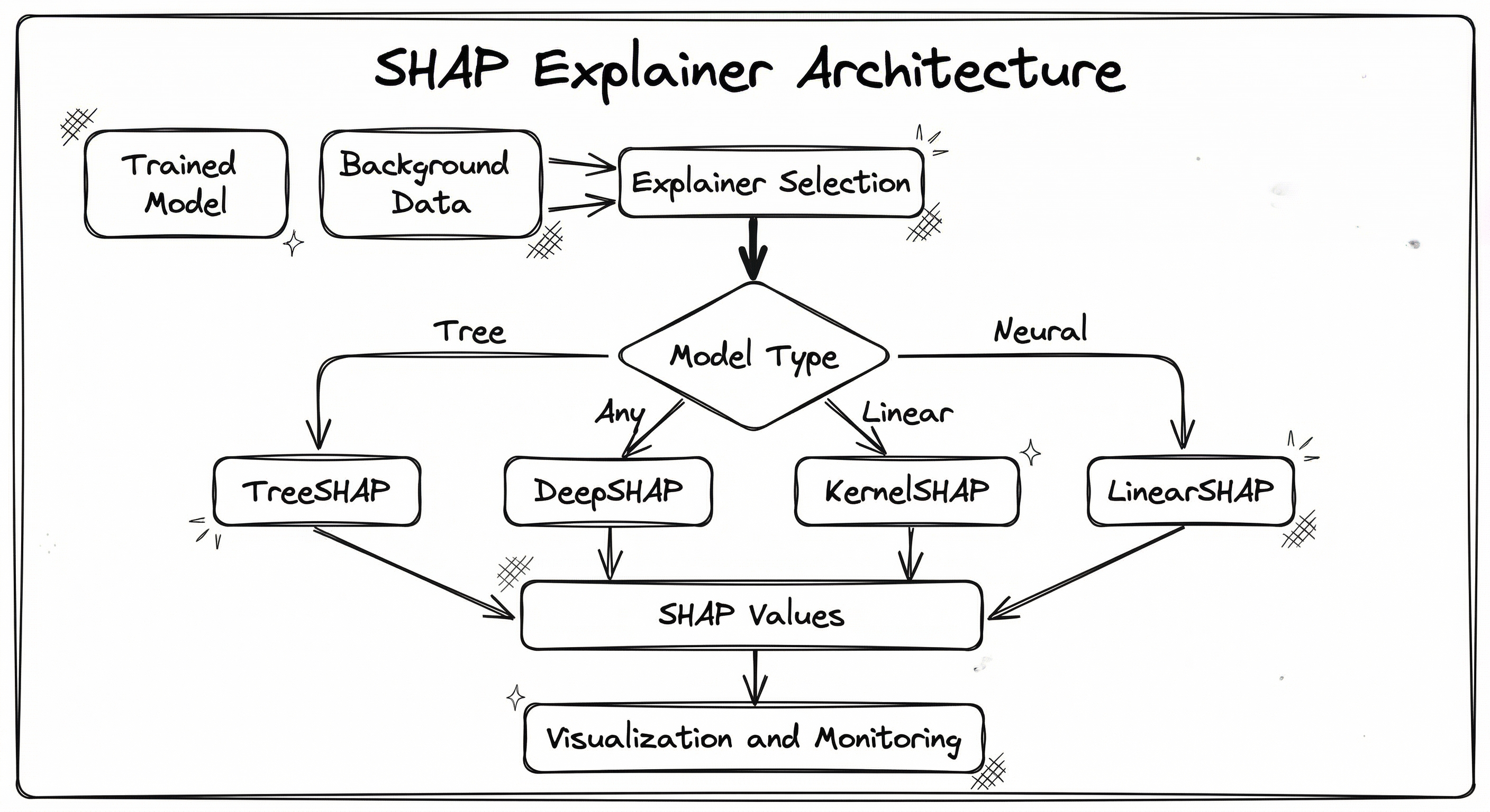
The architecture follows a strategy pattern: a single Explainer interface with specialized implementations that exploit model structure for computational efficiency. TreeSHAP can compute exact Shapley values in polynomial time by leveraging the tree structure, while KernelSHAP provides a model-agnostic fallback at higher computational cost.
Key Components
Explainer Selector
Inspects the model type and automatically selects the optimal SHAP algorithm. For sklearn.ensemble.GradientBoostingClassifier or xgboost.XGBClassifier, it routes to TreeSHAP. For torch.nn.Module or tensorflow.keras.Model, it routes to DeepSHAP. For anything else, it falls back to KernelSHAP.
Background Data Sampler
Selects a representative subset of the training data to serve as the baseline for marginalization. For KernelSHAP, the background dataset size directly affects both computation time and explanation quality. A common practice is k-means summarization to reduce background data to 50-100 representative points.
TreeSHAP Engine
Computes exact Shapley values for tree-based models (XGBoost, LightGBM, CatBoost, Random Forest, sklearn GBMs) by recursively traversing tree paths and tracking feature contributions. Runs in time -- polynomial, not exponential. Supports both interventional and tree-path-dependent (observational) feature perturbation.
KernelSHAP Engine
Model-agnostic Shapley value estimator using weighted linear regression over sampled feature coalitions. Treats the model as a black box, requiring only input-output access. Computationally expensive for high-dimensional inputs but works with any model type.
DeepSHAP Engine
Combines DeepLIFT's backpropagation-based attribution with Shapley value properties. Propagates SHAP values through each layer of a neural network by comparing neuron activations to reference activations. Faster than KernelSHAP for deep models but relies on an approximation that may not satisfy all Shapley axioms exactly.
Visualization Layer
Generates standardized SHAP plots: summary/beeswarm plots (global feature importance with distribution), waterfall plots (single-prediction decomposition), force plots (compact single-prediction view), dependence plots (feature value vs. SHAP value with interaction coloring), and bar plots (mean absolute SHAP values).
Monitoring & Audit Store
Persists SHAP values alongside predictions for regulatory auditing, drift detection, and historical explanation retrieval. In production systems (e.g., a lending platform), this enables answering queries like "why was loan application #12345 rejected 6 months ago?" -- a requirement under India's RBI Digital Lending Guidelines.
Data Flow
Explanation Path: A trained model and a data instance enter the explainer selector -> the appropriate SHAP algorithm is invoked with the background dataset -> the algorithm computes a SHAP value for each feature -> values are returned as a matrix of shape (n_instances, n_features) -> the visualization layer renders plots -> values are optionally persisted to the audit store.
Batch Explanation Path: For production monitoring, SHAP values are computed in batch (often offline or asynchronously) for a sample of predictions. These are aggregated into global importance rankings and drift dashboards. In latency-sensitive systems, SHAP computation runs on a separate pipeline from inference to avoid impacting prediction latency.
Real-time Explanation Path: For customer-facing explanations (e.g., "why was my loan rejected?"), SHAP values are pre-computed at inference time using TreeSHAP (which adds <5ms overhead for tree models) and stored alongside the prediction for instant retrieval.
A directed flowchart showing a Trained Model and Background Data feeding into the SHAP Explainer Selector, which branches based on model type to TreeSHAP, DeepSHAP, KernelSHAP, or LinearSHAP. All explainer branches converge into a SHAP Values Matrix, which feeds into both a Visualization Layer (producing summary, waterfall, force, and dependence plots) and a Monitoring/Audit Store.
How to Implement
Choosing Your Explainer
The SHAP library (maintained by Scott Lundberg) provides a unified Python API with specialized explainers. The selection rule is straightforward:
- Tree-based models (XGBoost, LightGBM, CatBoost, Random Forest, sklearn GBMs): Use
shap.TreeExplainer. It computes exact SHAP values in polynomial time. This is the fastest and most reliable option. - Deep neural networks (PyTorch, TensorFlow/Keras): Use
shap.DeepExplainerorshap.GradientExplainer. DeepSHAP is faster but approximate; GradientExplainer uses expected gradients and is more principled. - Any model (SVM, k-NN, custom models, API-based models): Use
shap.KernelExplainer. It only needs a prediction function, but is computationally expensive. For a model with 50 features and 100 background samples, expect 5-10 seconds per explanation. - Linear models (logistic regression, linear SVM): Use
shap.LinearExplainer. Computes exact SHAP values analytically using the model coefficients.
Production Considerations
In production, the key challenge is latency vs. explanation completeness. TreeSHAP adds negligible overhead (<5ms) and can be called inline during inference. KernelSHAP for a 100-feature model might take 10-30 seconds -- far too slow for real-time serving. The standard pattern is:
- Real-time models (tree-based): Compute SHAP values synchronously at inference time. Store alongside prediction.
- Complex models (deep learning, ensembles): Compute SHAP values asynchronously in a batch pipeline. Sample 1-5% of predictions for explanation.
- Regulatory audits: Pre-compute SHAP values for all predictions in the audit window. Store in a queryable format (Parquet, Delta Lake, or Azure Table Storage).
Cost Note: For a model serving 1 million predictions/day with KernelSHAP, computing SHAP values for a 1% sample (10,000 predictions) using a 4-vCPU VM on Azure takes approximately 8-12 hours and costs
INR 250-400/day ($3-5/day). TreeSHAP for the full 1 million predictions on the same VM takes under 30 minutes.
import xgboost as xgb
import shap
import pandas as pd
import numpy as np

# Load and train a credit scoring model
X_train = pd.read_csv("credit_train.csv")
y_train = X_train.pop("default")
model = xgb.XGBClassifier(
    n_estimators=500, max_depth=6, learning_rate=0.1,
    eval_metric="auc", use_label_encoder=False
)
model.fit(X_train, y_train)

# Create TreeSHAP explainer
explainer = shap.TreeExplainer(model)

# Compute SHAP values for a single applicant
applicant = X_train.iloc[[42]]
shap_values = explainer.shap_values(applicant)

# The base value (average model output on training data)
base_value = explainer.expected_value
print(f"Base value (avg prediction): {base_value:.4f}")
print(f"Model prediction: {model.predict_proba(applicant)[0][1]:.4f}")
print(f"Sum of SHAP + base: {base_value + shap_values[0].sum():.4f}")

# Generate explanation plots
shap.waterfall_plot(shap.Explanation(
    values=shap_values[0],
    base_values=base_value,
    data=applicant.values[0],
    feature_names=X_train.columns.tolist()
))

# Global feature importance across all training data
shap_values_all = explainer.shap_values(X_train)
shap.summary_plot(shap_values_all, X_train)
This example demonstrates the end-to-end SHAP workflow for a credit scoring model built with XGBoost. TreeSHAP computes exact Shapley values by exploiting the tree structure, running in time. The waterfall plot shows why a specific applicant was scored as they were, while the summary plot reveals global feature importance patterns. Notice how base_value + sum(shap_values) equals the model's prediction exactly -- this is the local accuracy property in action.
import shap
import numpy as np
from sklearn.ensemble import StackingClassifier
from sklearn.svm import SVC
from sklearn.linear_model import LogisticRegression
from sklearn.neural_network import MLPClassifier

# Assume a complex stacking ensemble (black-box)
stacked_model = StackingClassifier(
    estimators=[
        ("svm", SVC(probability=True)),
        ("mlp", MLPClassifier(hidden_layer_sizes=(100, 50))),
    ],
    final_estimator=LogisticRegression()
)
stacked_model.fit(X_train, y_train)

# KernelSHAP: summarize background data with k-means
background = shap.kmeans(X_train, 50)  # 50 cluster centroids

# Create model-agnostic explainer
explainer = shap.KernelExplainer(
    stacked_model.predict_proba,  # any callable
    background
)

# Explain a batch of instances (slow -- use sampling in production)
sample = X_test.iloc[:100]
shap_values = explainer.shap_values(sample, nsamples=500)

# Force plot for a single prediction
shap.force_plot(
    explainer.expected_value[1],
    shap_values[1][0],
    sample.iloc[0],
    matplotlib=True
)

# Dependence plot: how does "income" interact with "age"?
shap.dependence_plot("income", shap_values[1], sample, interaction_index="age")
KernelSHAP works with any model -- including stacking ensembles, SVMs, or even models behind an API. It treats the model as a black box, sampling feature coalitions and fitting a weighted linear model to estimate Shapley values. The nsamples parameter controls the accuracy-speed tradeoff: 500 samples gives reasonable approximations for most models, but increase to 2000+ for high-stakes applications. The k-means summarization of the background dataset reduces computation by 10-20x compared to using the full training set.
import torch
import torch.nn as nn
import shap
import numpy as np

# Define a simple neural network
class FraudDetector(nn.Module):
    def __init__(self, input_dim):
        super().__init__()
        self.layers = nn.Sequential(
            nn.Linear(input_dim, 128),
            nn.ReLU(),
            nn.BatchNorm1d(128),
            nn.Linear(128, 64),
            nn.ReLU(),
            nn.Dropout(0.3),
            nn.Linear(64, 1),
            nn.Sigmoid()
        )

    def forward(self, x):
        return self.layers(x)

# Train model (training code omitted for brevity)
model = FraudDetector(input_dim=30)
model.load_state_dict(torch.load("fraud_model.pt"))
model.eval()

# Select background data (reference inputs)
background = torch.tensor(X_train[:100].values, dtype=torch.float32)
test_data = torch.tensor(X_test[:10].values, dtype=torch.float32)

# Create DeepSHAP explainer
explainer = shap.DeepExplainer(model, background)
shap_values = explainer.shap_values(test_data)

# Visualize
shap.summary_plot(
    shap_values,
    X_test[:10],
    feature_names=feature_names,
    plot_type="bar"
)
DeepSHAP combines the DeepLIFT algorithm's backpropagation-based attribution with Shapley value theory. It propagates SHAP values layer-by-layer through the neural network, comparing each neuron's activation to its reference (background) activation. This is orders of magnitude faster than running KernelSHAP on a neural network. The tradeoff is that DeepSHAP makes a linearity assumption at each neuron that may not hold exactly for complex architectures -- but in practice, the approximation is very good for most feedforward and convolutional networks.
import shap
import json
import logging
from datetime import datetime
from typing import Dict, Any
import numpy as np

logger = logging.getLogger(__name__)

class SHAPExplanationService:
    """Production-grade SHAP explanation service with caching and audit logging."""

    def __init__(self, model, background_data, model_type="tree"):
        self.model_type = model_type
        if model_type == "tree":
            self.explainer = shap.TreeExplainer(model)
        elif model_type == "kernel":
            background = shap.kmeans(background_data, 50)
            self.explainer = shap.KernelExplainer(model.predict_proba, background)
        else:
            raise ValueError(f"Unsupported model type: {model_type}")

    def explain(self, instance: np.ndarray, feature_names: list) -> Dict[str, Any]:
        """Generate SHAP explanation for a single prediction."""
        start = datetime.utcnow()
        shap_values = self.explainer.shap_values(instance.reshape(1, -1))
        elapsed_ms = (datetime.utcnow() - start).total_seconds() * 1000

        # Handle binary classification (take positive class)
        if isinstance(shap_values, list):
            shap_values = shap_values[1]

        base_value = float(
            self.explainer.expected_value[1]
            if isinstance(self.explainer.expected_value, (list, np.ndarray))
            else self.explainer.expected_value
        )

        # Build explanation payload
        explanation = {
            "timestamp": datetime.utcnow().isoformat(),
            "base_value": base_value,
            "shap_values": {
                name: float(val)
                for name, val in zip(feature_names, shap_values[0])
            },
            "top_positive_features": sorted(
                [(name, float(val)) for name, val in zip(feature_names, shap_values[0]) if val > 0],
                key=lambda x: -x[1]
            )[:5],
            "top_negative_features": sorted(
                [(name, float(val)) for name, val in zip(feature_names, shap_values[0]) if val < 0],
                key=lambda x: x[1]
            )[:5],
            "computation_time_ms": round(elapsed_ms, 2),
            "explainer_type": self.model_type
        }

        logger.info(
            f"SHAP explanation generated in {elapsed_ms:.1f}ms "
            f"using {self.model_type} explainer"
        )
        return explanation

    def generate_rejection_reason(self, explanation: Dict) -> str:
        """Convert SHAP values to human-readable rejection reasons (RBI compliance)."""
        reasons = []
        for feature, value in explanation["top_negative_features"][:3]:
            reasons.append(
                f"Your {feature.replace('_', ' ')} negatively impacted "
                f"the decision (contribution: {value:.3f})"
            )
        return "; ".join(reasons)
This production-ready service wraps the SHAP library with logging, timing, and audit trail generation. The generate_rejection_reason method converts SHAP values into human-readable explanations suitable for customer-facing communications -- a direct requirement under RBI's Digital Lending Guidelines. In a real deployment, the explanation payload would be persisted to Azure Table Storage or a similar audit store for regulatory retrieval. Note the careful handling of binary classification SHAP value formats, which is a common source of bugs.
# SHAP explanation service configuration (YAML)
shap_config:
  default_explainer: tree
  tree_explainer:
    feature_perturbation: interventional
    model_output: raw  # or probability
  kernel_explainer:
    background_samples: 100
    nsamples: 1000
    l1_reg: auto
    summarize_method: kmeans  # or sample
  deep_explainer:
    background_samples: 100
  monitoring:
    sample_rate: 0.01  # explain 1% of predictions
    storage_backend: azure_table  # or parquet, delta_lake
    retention_days: 365
    alert_on_drift: true
    drift_threshold: 0.15  # alert if mean |SHAP| shift > 15%
  visualization:
    default_plots:
      - summary
      - waterfall
    max_display_features: 20
    color_scheme: coolwarm
Common Implementation Mistakes
- ●
Using the wrong background dataset: KernelSHAP and DeepSHAP require a background dataset to marginalize absent features. Using a random subset that does not represent the data distribution (e.g., only including approved loans in a credit model's background) biases all SHAP explanations. Always use a stratified sample of the training data, or use
shap.kmeans()for efficient summarization. - ●
Confusing TreeSHAP's interventional vs. observational mode: TreeSHAP supports two feature perturbation methods. The default
feature_perturbation='tree_path_dependent'uses the tree structure itself to marginalize features, which can introduce bias when features are correlated. For causal-style explanations, usefeature_perturbation='interventional'with explicit background data. - ●
Computing SHAP values on raw model output vs. probability: For classification models, SHAP values can be computed on the raw logit, log-odds, or probability scale. Computing on probability scale makes values non-additive in the probability space (due to the sigmoid nonlinearity). Prefer computing on the log-odds scale and converting to probability only for presentation.
- ●
Ignoring SHAP value stability across runs: KernelSHAP is a sampling-based estimator. Two runs with different random seeds will produce slightly different SHAP values. For regulatory submissions, fix the random seed and use sufficient samples (nsamples >= 1000). Report confidence intervals when possible.
- ●
Treating SHAP values as causal effects: SHAP values measure feature contribution to a prediction, not causal impact. A high SHAP value for "zip code" in a loan model does not mean changing the applicant's zip code would change the outcome. SHAP captures correlation-based attribution, not counterfactual causation.
- ●
Not normalizing input features before KernelSHAP: KernelSHAP fits a local linear model. Features on vastly different scales can cause numerical instability in the weighted regression. Always use the same preprocessing (scaling, encoding) that the original model expects.
When Should You Use This?
Use When
You need mathematically rigorous feature attributions with axiomatic guarantees (consistency, local accuracy, missingness) -- not ad-hoc importance scores
Regulatory requirements mandate explanation of individual model decisions (EU AI Act Article 13, RBI Digital Lending Guidelines, US SR 11-7)
You want both local (per-prediction) and global (aggregate) interpretability from a single framework
Your model is a tree ensemble (XGBoost, LightGBM, CatBoost, Random Forest) where TreeSHAP provides exact values with negligible computational overhead
You need to compare feature importance across different model types on a common scale (e.g., comparing a gradient-boosted model vs. a neural network)
Model debugging: identifying why specific predictions are wrong, detecting data leakage via unexpected feature importances, or diagnosing distribution shift
Fairness auditing: measuring the contribution of protected attributes (gender, caste, religion, age) to model predictions to detect algorithmic bias
Avoid When
Your model is extremely high-dimensional (>1000 features) and you need real-time explanations -- KernelSHAP will be too slow, and even TreeSHAP may struggle with very wide trees. Consider dimensionality reduction first.
You need causal explanations, not attributional ones. SHAP tells you what the model used, not what would happen if you intervened. Use causal inference methods (DoWhy, CausalML) instead.
Your model is a simple linear regression or logistic regression where coefficients are already interpretable. SHAP adds overhead without additional insight -- just read the coefficients.
Latency budget is <1ms and the model is not tree-based. KernelSHAP and DeepSHAP add 100ms-30s of overhead. For sub-millisecond explanations, use model-intrinsic interpretability (attention weights, linear probes).
You only need global feature importance rankings and do not need per-prediction explanations. Permutation importance or built-in feature importance is simpler and faster.
The model operates on unstructured data (raw images, audio waveforms) where per-pixel/per-sample SHAP values are not meaningful to end-users. Use GradCAM, attention visualization, or concept-based explanations instead.
Key Tradeoffs
Exactness vs. Speed
The fundamental tradeoff in SHAP is between exact computation and computational cost. TreeSHAP gives you exact values for free (milliseconds per prediction). KernelSHAP gives you approximate values for any model at 1000-10000x the cost. DeepSHAP sits in between: fast but not perfectly exact.
For production systems, this means tree-based models get a "free lunch" -- you can explain every prediction in real time. For deep learning models, you typically explain a sample offline.
Interventional vs. Observational
TreeSHAP offers two modes:
| Mode | Marginalizes via | Handles correlations? | Causal interpretation? |
|---|---|---|---|
| Tree-path-dependent (default) | Tree structure | No (ignores feature correlations) | No |
| Interventional | Background data | Yes (respects data distribution) | Closer to causal |
The tree-path-dependent mode is faster and does not require background data, but can produce misleading attributions when features are correlated (e.g., attributing importance to correlated features that the model doesn't directly use). For correlated features, interventional mode is safer.
Fidelity vs. Interpretability
SHAP values are perfectly faithful to the model (they decompose the exact prediction), but they may not be interpretable to non-technical users. A SHAP value of -0.032 for "debt_to_income_ratio" is precise but not meaningful to a loan applicant. Production systems need a translation layer that converts SHAP values into natural language explanations (e.g., "Your debt-to-income ratio of 0.65 is higher than 85% of approved applicants, which decreased your approval score").
Cost Comparison: Computing SHAP values for 1 million predictions using TreeSHAP on a standard 4-vCPU Azure VM (D4s_v3, ~INR 7,500/month or ~1,800) per run. This 1000x cost difference is why model architecture choice has direct implications for your explainability budget.
Alternatives & Comparisons
LIME generates local explanations by fitting a simple interpretable model (typically linear regression) in the neighborhood of a prediction. LIME is faster than KernelSHAP and more intuitive for non-technical audiences, but it lacks SHAP's axiomatic guarantees -- LIME explanations can be inconsistent (changing the neighborhood size changes the explanation). Choose LIME when speed matters more than mathematical rigor, or when explaining to business stakeholders who prefer simpler narratives. Choose SHAP when you need provably consistent attributions, especially for regulatory submissions.
Bias detectors identify systematic disparities in model predictions across protected groups (gender, caste, age, etc.), while SHAP explains individual predictions at the feature level. They are complementary: SHAP can tell you why a specific prediction was biased (e.g., high SHAP value for a proxy feature like zip code), while a bias detector tells you that the model is biased across a population. Use both in a comprehensive responsible AI pipeline.
Fairness checkers evaluate metrics like demographic parity, equalized odds, and calibration across groups. SHAP provides the mechanistic explanation of how features drive predictions. A fairness checker might flag that female applicants are rejected 20% more often; SHAP reveals that the model is over-weighting "years of experience" which correlates with gender. Choose a fairness checker for population-level auditing; choose SHAP for understanding the feature-level mechanism behind disparities.
For deep learning models, integrated gradients and attention-based explanations are computed during the forward/backward pass and are tightly coupled to the model architecture. They are faster than DeepSHAP and naturally align with the model's computation. However, they lack Shapley value's axiomatic properties -- attention weights, in particular, have been shown to not reliably indicate feature importance (Jain & Wallace, 2019). Choose model-intrinsic methods when latency is critical and axiomatic guarantees are not required; choose SHAP when you need theoretically grounded attributions.
Pros, Cons & Tradeoffs
Advantages
Axiomatic foundation: SHAP is the only feature attribution method backed by the full set of Shapley value axioms (efficiency, symmetry, dummy, additivity). This is not a marketing claim -- it is a mathematical theorem.
Unified local + global interpretability: Aggregate local SHAP values to get global feature importance. No other method provides both perspectives from a single computation.
Model-agnostic with model-specific accelerations: KernelSHAP works with any model, while TreeSHAP and DeepSHAP exploit model structure for orders-of-magnitude speedups. You never hit a dead end.
Rich visualization ecosystem: Summary plots, waterfall plots, force plots, dependence plots, and interaction plots provide multiple complementary views of model behavior out of the box.
Regulatory acceptance: SHAP is explicitly cited in regulatory guidance documents, model risk management frameworks, and academic literature as the gold standard for feature attribution. Using SHAP significantly de-risks regulatory reviews.
Exact for tree models: TreeSHAP computes exact Shapley values in polynomial time for the most popular production model family (gradient-boosted trees). No approximation, no sampling error.
Interaction effects: SHAP interaction values decompose feature contributions into main effects and pairwise interactions, revealing non-obvious feature synergies that global importance misses.
Disadvantages
Exponential worst-case complexity: For model-agnostic computation (KernelSHAP), the cost scales as where is the number of features and is the number of samples. For 500+ features, even sampling-based approximation becomes prohibitively expensive.
Not causal: SHAP values reflect correlational attribution, not causal effects. In the presence of multicollinearity, SHAP may distribute importance across correlated features in non-intuitive ways -- leading to spurious conclusions if interpreted causally.
Background data sensitivity: KernelSHAP and DeepSHAP results depend on the choice of background (reference) dataset. A poorly chosen background can produce misleading explanations. There is no universally "correct" background.
Explanation instability for KernelSHAP: Because KernelSHAP uses random sampling, explanations vary between runs. For high-stakes applications (credit, healthcare), this non-determinism can be problematic. You must fix seeds and use sufficient samples.
Cognitive overload for high-dimensional models: A SHAP explanation for a model with 200 features produces 200 numbers per prediction. Without careful UI design and aggregation, this overwhelms rather than clarifies. Translation to natural language is essential but non-trivial.
DeepSHAP approximation quality: DeepSHAP's layer-wise propagation makes a linearization assumption that may not hold for architectures with complex skip connections, attention mechanisms, or non-standard activations. Verification against KernelSHAP is recommended for novel architectures.
Failure Modes & Debugging
Correlated feature attribution leakage
Cause
When features are highly correlated (e.g., total_income and monthly_salary), SHAP distributes importance across both features. In tree-path-dependent mode, TreeSHAP may even attribute importance to features the model doesn't directly split on, because the tree structure implicitly conditions on correlated features.
Symptoms
Seemingly irrelevant features appear with non-zero SHAP values. Domain experts flag explanations as "wrong" because a feature they know is irrelevant shows up as important. Explanations differ significantly between interventional and tree-path-dependent modes.
Mitigation
Use interventional TreeSHAP (feature_perturbation='interventional') with a representative background dataset. Alternatively, perform feature selection to remove redundant correlated features before training. Report SHAP values for feature groups (e.g., "income-related features") rather than individual features when correlation is unavoidable.
Background data distribution mismatch
Cause
KernelSHAP marginalizes absent features by replacing them with values from the background dataset. If the background data is not representative of the population (e.g., using only approved loans as background for a loan model), SHAP values are computed against a biased reference and produce misleading explanations.
Symptoms
SHAP base value does not match the model's average prediction on the target population. Feature attributions seem systematically skewed in one direction. Adding a new background dataset changes all explanations significantly.
Mitigation
Always use a stratified, representative sample of the training data as background. Validate that the base value matches the model's average prediction on a hold-out set. Use shap.kmeans() to create a compact, representative summary. Document the background dataset choice in your model card.
Computational timeout in production
Cause
KernelSHAP called synchronously in the inference path for a model with many features or a slow prediction function. Each SHAP computation requires hundreds to thousands of model evaluations.
Symptoms
API latency spikes from <100ms to 10-30 seconds. Request timeouts. Cascading failures in downstream services waiting for explanations. SLA violations.
Mitigation
Never run KernelSHAP synchronously in the inference path. Use TreeSHAP for tree models (adds <5ms). For other models, compute SHAP asynchronously: return the prediction immediately, enqueue explanation computation, and serve explanations via a separate endpoint. Use caching for repeated similar inputs.
SHAP value drift without model retraining
Cause
Input data distribution shifts over time (concept drift), causing SHAP values to change even though the model is static. Features that were previously unimportant become dominant, or vice versa.
Symptoms
Monitoring dashboards show gradual shift in mean SHAP values for key features. Explanations for similar-looking inputs differ significantly across time periods. Regulatory auditors flag inconsistencies in historical vs. current explanations.
Mitigation
Track SHAP value distributions over time using statistical tests (KS test, PSI). Set alerts when the mean absolute SHAP value for any feature shifts by more than 15-20% relative to the baseline period. SHAP drift is often an early warning signal of model degradation -- use it to trigger model retraining.
Misinterpretation as causal explanation
Cause
Stakeholders (product managers, compliance officers, customers) interpret SHAP values as causal statements: "the model rejected you because of your low income." In reality, SHAP measures attributional contribution, not causal effect.
Symptoms
Business decisions made based on SHAP values lead to unexpected outcomes. For example, a bank tells applicants to "increase their credit limit to improve approval chances" based on SHAP values, but the credit limit is a downstream effect of creditworthiness, not a cause.
Mitigation
Always accompany SHAP explanations with a disclaimer: "These values indicate how features contributed to this specific prediction, not how changing these features would change the outcome." Train stakeholders on the distinction between attribution and causation. For causal questions, use dedicated causal inference tools (DoWhy, EconML).
Adversarial manipulation of SHAP explanations
Cause
An adversary crafts model inputs specifically to produce misleading SHAP explanations -- hiding the true decision-making feature behind correlated proxies. Research has shown it is possible to train models that produce plausible-looking SHAP explanations while actually relying on different features (Slack et al., 2020).
Symptoms
SHAP explanations pass human review but the model is actually using protected attributes via proxy features. Fairness audits based solely on SHAP values give a false sense of safety.
Mitigation
Never rely on SHAP alone for fairness auditing. Combine SHAP with counterfactual explanations, partial dependence plots, and group-level fairness metrics. Use adversarial testing to probe whether explanations are robust to perturbations. Audit the model's behavior, not just its explanations.
Placement in an ML System
Where SHAP Sits in the ML System
SHAP operates as a post-hoc explanation layer that consumes trained models and their predictions. It does not modify the model or its predictions in any way -- it only adds interpretability metadata.
In a typical production pipeline:
-
Training phase: After model training completes, SHAP is used to compute global feature importance on the validation set. This informs feature selection, model debugging, and documentation for model review committees.
-
Serving phase: For tree-based models, SHAP values are computed inline during inference (adding <5ms latency). For complex models, SHAP runs asynchronously on a sample of predictions. The explanation payloads are stored alongside predictions in the audit store.
-
Monitoring phase: SHAP value distributions are tracked over time. Drift in SHAP values (without model retraining) signals input distribution shift. Sudden changes in which features dominate explanations can indicate data quality issues, adversarial inputs, or concept drift.
-
Compliance phase: Regulators and auditors query the SHAP audit store to review explanations for specific decisions. In India, this is particularly relevant for lending (RBI), insurance (IRDAI), and healthcare AI systems.
Integration Point: SHAP explanations feed directly into bias detectors and fairness checkers -- if the SHAP value for a protected attribute (or its proxy) is systematically high, it triggers bias alerts downstream.
Pipeline Stage
Post-Training / Serving / Monitoring
Upstream
- model-training
- feature-store
Downstream
- bias-detector
- fairness-checker
- model-monitoring
Scaling Bottlenecks
The primary bottleneck is the computational cost of SHAP value estimation, which varies enormously by explainer type:
- TreeSHAP: Scales linearly with the number of predictions. 1M explanations for a 500-tree XGBoost model takes ~20-30 minutes on a single machine. GPU-accelerated TreeSHAP (NVIDIA GPUTreeSHAP) can reduce this to under 2 minutes.
- KernelSHAP: Scales quadratically with features and linearly with sample count. For a 100-feature model with 1000 samples, each explanation takes 5-15 seconds. Computing 1M explanations would require ~5,000 CPU-hours (~INR 4 lakh or ~$480 on Azure spot instances).
- Storage: Each explanation produces a vector of M float values per prediction. For a 100-feature model and 1M daily predictions, that is 100M floats/day = ~400MB/day in raw storage, or ~12GB/month. With metadata, expect 20-30GB/month for audit storage.
The scaling pattern is: use TreeSHAP for real-time explanation of tree models, use KernelSHAP/DeepSHAP for offline batch explanation of complex models, and use GPU acceleration (RAPIDS GPUTreeSHAP) when throughput requirements exceed single-CPU capacity.
Production Case Studies
NVIDIA developed GPU-accelerated SHAP (GPUTreeSHAP) to enable real-time explainability for credit risk models at scale. Their implementation uses massively parallel CUDA kernels to compute exact TreeSHAP values, flattening millions of tree paths and mapping them to thousands of GPU cores. The system was demonstrated on mortgage delinquency prediction models, achieving up to 340x speedup over CPU-based SHAP for interaction values.
GPU-accelerated SHAP computation reduced explanation time for a 1000-tree XGBoost model from hours to seconds, making real-time per-decision explainability feasible for financial institutions processing millions of credit applications daily. Cost per explanation dropped from approximately 0.00001.
Indeed's Interview team used SHAP decision plots to identify which features most impacted candidate-employer matching quality. By analyzing SHAP values across thousands of predictions, they identified high-impact A/B test hypotheses -- replacing manual intuition with data-driven experiment design. The team used SHAP summary plots to prioritize which product features to test first.
SHAP-driven A/B test selection led to a 5-10% increase in key business metrics by focusing experimentation resources on the features that SHAP identified as most impactful, rather than relying on domain intuition alone.
Uber's engineering blog details their model explainability framework that relies heavily on local feature attributions for individual predictions, such as pinpointing whether location or time played the biggest role when flagging a trip as potentially fraudulent. The framework is designed to be extensible, incorporating methods including SHAP and DeepLIFT with minimal engineering effort.
Enables fraud teams to understand model decisions with feature-level explanations, improving trust and actionability in real-time fraud detection systems across Uber's global operations.
The UK Government's AI Assurance portfolio includes SHAP-based explainability as a recommended technique for AI systems in regulated sectors. Their case study demonstrates applying accelerated SHAP computation to credit risk management, highlighting how Shapley values provide a mathematically grounded method for regulators to verify that AI lending decisions are transparent and non-discriminatory.
Established SHAP as a government-endorsed AI assurance technique, providing a framework for financial institutions in the UK and internationally to demonstrate regulatory compliance for AI-powered credit decisions.
Tooling & Ecosystem
The official SHAP library by Scott Lundberg. Provides TreeExplainer, KernelExplainer, DeepExplainer, GradientExplainer, LinearExplainer, and PermutationExplainer. Includes a rich visualization suite (summary, waterfall, force, dependence, interaction plots). The de facto standard for Shapley-based model explanation.
LinkedIn's optimized implementation of TreeSHAP that achieves 1.5-2.5x speedup over the standard SHAP library's TreeExplainer through algorithmic optimizations (Fast TreeSHAP v1 and v2). Drop-in replacement for shap.TreeExplainer with identical outputs.
NVIDIA RAPIDS' GPU-accelerated TreeSHAP implementation. Uses massively parallel CUDA kernels to compute exact SHAP values, achieving up to 20x speedup for SHAP values and 340x speedup for SHAP interaction values over CPU-based computation. Integrated with XGBoost's pred_contribs parameter.
Microsoft's open-source interpretability toolkit that includes SHAP alongside other explanation methods (EBM, LIME, Morris sensitivity). Provides a unified dashboard for comparing explanations across methods. Useful for regulatory audits where multiple explanation techniques are required.
R package for creating publication-quality SHAP visualizations. Supports waterfall, beeswarm, force, dependence, and interaction plots with ggplot2 integration. Ideal for teams using R for statistical analysis and reporting.
Seldon's open-source library for ML model inspection and interpretation. Includes KernelSHAP alongside counterfactual explanations, anchors, and integrated gradients. Integrates with Seldon Core for production model serving with explanations.
India-based enterprise XAI platform that provides SHAP-based explanations with regulatory compliance reporting for Indian financial institutions. Offers pre-built compliance templates for RBI and IRDAI requirements, with automated explanation generation and audit trails.
Research & References
Lundberg, S.M. & Lee, S.-I. (2017)NeurIPS 2017
The foundational SHAP paper that unified six existing interpretability methods (LIME, DeepLIFT, LRP, Shapley regression, Shapley sampling, QII) under the Shapley value framework. Introduced KernelSHAP and proved that Shapley values are the unique solution satisfying local accuracy, missingness, and consistency.
Lundberg, S.M., Erion, G.G. & Lee, S.-I. (2019)Nature Machine Intelligence, Vol. 2
Introduced TreeSHAP -- the polynomial-time exact Shapley value algorithm for tree-based models. Demonstrated that standard feature importance measures for trees (Gini, split count) can be inconsistent, while TreeSHAP provides provably consistent attributions. Reduced complexity from to .
Lundberg, S.M., Erion, G., Chen, H., DeGrave, A., Prutkin, J.M., Nair, B., Katz, R., Himmelfarb, J., Bansal, N. & Lee, S.-I. (2020)Nature Machine Intelligence, Vol. 2
Extended SHAP to provide global model understanding through aggregation of local explanations. Introduced SHAP interaction values and demonstrated their use in identifying non-linear feature interactions in healthcare models.
Yang, J. (2021)NeurIPS 2021 XAI4Debugging Workshop
Proposed two algorithmic improvements (Fast TreeSHAP v1 and v2) that accelerate TreeSHAP computation by 1.5-2.5x while maintaining exact computation. The v2 algorithm trades slightly higher memory usage for significant speedup. Released as LinkedIn's open-source FastTreeSHAP library.
Slack, D., Hilgard, S., Jia, E., Singh, S. & Lakkaraju, H. (2020)AAAI/ACM AIES 2020
Demonstrated that SHAP (and LIME) can be fooled by adversarial classifiers that produce plausible explanations while hiding discriminatory behavior. This important negative result established that SHAP explanations alone are insufficient for fairness auditing -- complementary methods are necessary.
Mitchell, R., Frank, E. & Holmes, G. (2022)PeerJ Computer Science
Presented a massively parallel GPU algorithm for exact TreeSHAP computation. Achieves up to 340x speedup for SHAP interaction values by flattening tree paths and mapping dynamic programming to CUDA cores. Underlies NVIDIA RAPIDS' GPUTreeSHAP implementation.
Nguyen, C., Zelch, I. & Zivkovic, M. (2024)arXiv preprint
Explores using LLMs to translate raw SHAP values into natural language explanations accessible to non-technical users. Demonstrates that GPT-4 can generate clinically meaningful narratives from SHAP outputs in healthcare applications, bridging the gap between mathematical attribution and human understanding.
Interview & Evaluation Perspective
Common Interview Questions
- ●
What are Shapley values and why are they used in ML interpretability?
- ●
Explain the difference between TreeSHAP, KernelSHAP, and DeepSHAP. When would you use each?
- ●
What are the computational complexity tradeoffs between exact Shapley values and approximation methods?
- ●
How would you deploy SHAP explanations in a production credit scoring system?
- ●
Can SHAP values be used for causal inference? What are the limitations?
- ●
How would you handle SHAP explanations when features are highly correlated?
- ●
Describe a scenario where SHAP explanations could be misleading. How would you mitigate this?
- ●
How does SHAP relate to regulatory requirements like the EU AI Act or RBI Digital Lending Guidelines?
Key Points to Mention
- ●
SHAP is the unique attribution method satisfying all four Shapley axioms (efficiency, symmetry, dummy, additivity). Start with this -- it establishes why SHAP is theoretically superior to alternatives like feature importance or LIME.
- ●
TreeSHAP provides exact Shapley values in time for tree ensembles -- the only practical exact solution for non-trivial models. Mention the specific complexity, not just "it's fast."
- ●
The base value anchoring property: SHAP values sum to
prediction - E[f(X)]. This means explanations are a complete, additive decomposition of the prediction with zero residual. - ●
Interventional vs. tree-path-dependent TreeSHAP: the default mode can be misleading for correlated features. Interventional mode is safer but requires background data. This nuance separates senior candidates from junior ones.
- ●
SHAP is attributional, not causal. A high SHAP value for feature X means the model relied on X, not that intervening on X would change the outcome. Always clarify this distinction.
- ●
GPU acceleration (RAPIDS GPUTreeSHAP) achieves 20-340x speedups and is essential for production systems processing millions of predictions. Mention specific numbers.
Pitfalls to Avoid
- ●
Claiming SHAP provides causal explanations -- it does not. SHAP measures feature attribution within the model, not real-world causal effects. This is the #1 conceptual mistake in interviews.
- ●
Saying "SHAP is slow" without qualifying which explainer. TreeSHAP adds <5ms per prediction. KernelSHAP is slow. The distinction matters enormously.
- ●
Ignoring the background data requirement and its impact on explanations. The choice of background dataset is a design decision that affects all explanations -- not a minor implementation detail.
- ●
Treating SHAP as a silver bullet for model interpretability. SHAP explains what the model does, not whether the model is right. It can perfectly explain a terrible model.
- ●
Confusing global feature importance (mean |SHAP|) with local SHAP values. They serve different purposes and should be discussed separately.
Senior-Level Expectation
A senior/staff-level candidate should discuss the full production lifecycle of SHAP: choosing the right explainer based on model type and latency requirements, computing and persisting SHAP values at scale (batch vs. real-time), monitoring SHAP distributions for drift, translating SHAP values into natural language for customer-facing explanations, and integrating SHAP into regulatory compliance workflows (model cards, audit trails, adverse action notices).
Expect them to articulate the limitations clearly: correlated feature attribution leakage, background data sensitivity, adversarial manipulation (Slack et al., 2020), and the fundamental non-causality of SHAP. They should propose mitigations for each.
A truly senior candidate will discuss cost-performance optimization: using GPU-accelerated TreeSHAP for high-throughput scenarios, sampling strategies for KernelSHAP in production, and the architecture of an async explanation pipeline that decouples inference latency from explanation computation. They should be able to estimate costs: for a model serving 10 million predictions/day in India, what does it cost to explain all of them (TreeSHAP: INR 250/day) vs. 1% of them with KernelSHAP ( INR 15,000/day)?
Summary
What We Covered
SHAP (SHapley Additive exPlanations) is the gold standard for model-agnostic, axiomatically grounded feature attribution in machine learning. Rooted in Shapley values from cooperative game theory -- a concept with 70+ years of mathematical justification -- SHAP uniquely satisfies local accuracy (explanations sum to the prediction), consistency (monotonic attribution updates), and missingness (absent features get zero attribution). No other feature attribution method provides all three guarantees simultaneously.
The practical ecosystem revolves around three key algorithms: TreeSHAP for exact, polynomial-time explanations of tree ensembles (the workhorse of production ML); DeepSHAP for efficient neural network explanations via backpropagation; and KernelSHAP as the model-agnostic fallback for anything else. The computational cost ranges from negligible (<5ms per prediction for TreeSHAP) to substantial (10+ seconds per prediction for KernelSHAP), making model architecture choice directly impact your explainability budget.
In production, SHAP serves three critical functions: debugging (why is the model making this specific mistake?), compliance (providing feature-level explanations for regulatory audits under the EU AI Act, RBI guidelines, and US model risk management standards), and monitoring (tracking SHAP distributions over time to detect concept drift and data quality issues). The combination of TreeSHAP's speed, GPU acceleration via NVIDIA GPUTreeSHAP, and rich visualization tools makes SHAP deployable at scale -- from a Bengaluru fintech serving thousands of loan decisions daily to a global bank processing millions of credit applications.
Remember: SHAP explains what the model did, not what should be done. It is a diagnostic tool, not a prescriptive one. Pair it with fairness checkers, bias detectors, and causal inference tools for a comprehensive responsible AI pipeline.