Explainer (LIME) in Machine Learning
LIME -- Local Interpretable Model-agnostic Explanations -- is one of the most influential techniques in the explainable AI (XAI) toolbox. It answers a deceptively simple question: why did the model make this particular prediction? And it does so without requiring any knowledge of the model's internal architecture.
The core idea is elegant: to explain a single prediction, LIME perturbs the input, observes how the black-box model's output changes, and fits a simple, interpretable surrogate model (typically a sparse linear model) in the local neighborhood of that prediction. The surrogate model's coefficients then serve as human-readable feature importances.
LIME occupies a critical position in the responsible AI stack. In regulated industries -- banking (think RBI's FREE-AI framework in India), healthcare diagnostics, and insurance underwriting -- stakeholders increasingly demand per-prediction explanations, not just global feature importances. LIME delivers exactly that: instance-level, model-agnostic explanations that can be generated for any classifier or regressor, whether it is a gradient-boosted tree, a deep neural network, or a black-box API endpoint.
Since its introduction by Ribeiro, Singh, and Guestrin in 2016 at KDD, the original paper has accumulated over 11,000 citations, spawned an active open-source library, and inspired a family of improved variants (S-LIME, BayLIME, Anchor explanations). Understanding LIME is foundational for any ML engineer building trustworthy, auditable systems.
Concept Snapshot
- What It Is
- A perturbation-based, model-agnostic explanation method that approximates any black-box model's behavior locally around a single prediction using an interpretable surrogate model.
- Category
- Responsible AI
- Complexity
- Intermediate
- Inputs / Outputs
- Inputs: a trained model (any framework), a single instance to explain, and the model's prediction function. Outputs: per-feature importance weights indicating each feature's contribution to that specific prediction.
- System Placement
- Sits in the post-prediction / model audit stage of the ML pipeline, after inference and before human review, compliance reporting, or downstream decision-making.
- Also Known As
- Local Interpretable Model-agnostic Explanations, LIME explainer, local surrogate model, perturbation-based explainer
- Typical Users
- ML Engineers, Data Scientists, Model Risk Analysts, Compliance Officers, Product Managers
- Prerequisites
- Supervised learning fundamentals (classification/regression), Linear regression basics, Feature importance concepts, Basic probability (sampling, distributions)
- Key Terms
- local fidelityperturbationsurrogate modelkernel widthinterpretable representationsparse linear modelsuperpixelbag-of-wordsexponential kernelmodel-agnostic
Why This Concept Exists
The Black-Box Problem
Modern ML models are powerful precisely because they are complex. Gradient-boosted ensembles with thousands of trees, deep neural networks with millions of parameters, transformer-based LLMs with billions of weights -- these models achieve state-of-the-art accuracy by learning intricate, non-linear decision boundaries that no human can inspect directly.
But this power comes at a cost: opacity. When a credit-scoring model denies a loan application at HDFC Bank, the applicant has a legal right to know why. When a diagnostic CNN flags a chest X-ray as positive for pneumonia at AIIMS, the radiologist needs to understand which regions the model focused on. When a fraud detection system at Razorpay blocks a transaction, the merchant needs a reason.
Before LIME, the options were limited. You could use inherently interpretable models (logistic regression, small decision trees), sacrificing accuracy. Or you could use complex models and accept that their decisions were opaque. LIME broke this dichotomy.
The Key Insight: Local Simplicity
The foundational insight behind LIME is that even if a model's global decision boundary is impossibly complex, the local behavior around any single prediction can often be well-approximated by a simple, interpretable model. Think of it like the surface of the Earth: globally, it is a complex, irregular geoid. But locally -- say, within your neighborhood -- it looks flat. A flat plane is a perfectly good approximation at that scale.
LIME exploits this by fitting a linear model in the neighborhood of the instance being explained. The linear model is wrong globally (it cannot capture the full complexity of the black box), but it is faithful locally -- and that is all we need for a single-instance explanation.
Regulatory Tailwinds
The importance of LIME has only grown with the wave of AI regulation worldwide. The EU AI Act (2024) mandates explanations for high-risk AI systems. India's RBI FREE-AI framework (2025) explicitly names interpretation tools like SHAP and LIME as mechanisms for achieving "Understandable by Design" AI in financial services. SEBI's AI-Use Rulebook (2025) demands algorithmic transparency in trading and underwriting.
In this regulatory landscape, LIME is not just a nice-to-have research tool -- it is a compliance requirement. Teams at Indian fintech companies like Razorpay, Lendingkart, and Paytm are actively integrating LIME into their model governance pipelines to meet these mandates.
Key Takeaway: LIME exists because we need per-prediction explanations for complex models, and it achieves this by recognizing that global complexity does not preclude local simplicity.
Core Intuition & Mental Model
The Coffee-Shop Explanation
Imagine you have a friend who is a brilliant but eccentric chef. You ask them why they added saffron to a particular biryani. Instead of explaining their entire culinary philosophy (which would take hours), they say: "For this specific dish, the saffron was the most important addition because the meat was mild and needed an aromatic lift. The yogurt mattered too, but less. The salt was negligible."
That is exactly what LIME does. It does not try to explain the entire model (the chef's full philosophy). It explains one specific prediction (this particular biryani) by identifying which input features (ingredients) mattered most for that output.
The Three-Step Dance
LIME performs a conceptually simple three-step process for every explanation:
-
Perturb: Generate a set of "neighbor" instances by slightly modifying the original input. For tabular data, this means toggling features on and off or sampling from their distributions. For text, it means randomly removing words. For images, it means masking groups of pixels (superpixels).
-
Predict: Feed each perturbed instance through the black-box model and record the predictions. This tells us how the model responds to changes in the input.
-
Fit a surrogate: Weight the perturbed instances by their proximity to the original (closer neighbors matter more), then fit a simple interpretable model -- typically a weighted sparse linear regression -- on these (perturbed input, prediction) pairs. The resulting coefficients are the explanation.
The beauty of this approach is its universality. LIME never looks inside the model. It only needs the ability to call the model's predict() function. This is why it works on scikit-learn classifiers, TensorFlow models, PyTorch networks, and even black-box API endpoints like Azure OpenAI.
The Locality Knob
How "local" is local? This is controlled by the kernel width parameter, which determines how much weight distant neighbors receive. A small kernel width means LIME focuses on a very tight neighborhood (high local fidelity but potentially noisy). A large kernel width means LIME considers a broader region (smoother explanations but potentially lower local fidelity). Tuning this parameter is one of the key practical challenges, and we will discuss it in depth in the implementation section.
Mental Model: LIME is like using a magnifying glass on a complex painting. The magnifying glass (kernel width) determines how much of the painting you see. Zoom in too much and you see noise in the brushstrokes. Zoom out too much and you lose the detail of the specific region you care about.
Technical Foundations
Mathematical Framework
Let denote the black-box model we wish to explain, and let be the instance whose prediction we want to interpret. LIME seeks an explanation model , where is a class of interpretable models (e.g., linear models, short decision trees).
The explanation is obtained by solving the following optimization problem:
where:
- is a fidelity loss measuring how well approximates in the neighborhood of , weighted by the proximity kernel
- is a complexity penalty that encourages interpretability (e.g., limiting the number of non-zero coefficients in a linear model)
The Proximity Kernel
The locality is defined by an exponential kernel:
where is a distance function (typically Euclidean for tabular data, cosine for text) between the original instance and a perturbed sample , and is the kernel width parameter.
This kernel assigns weights close to 1 for perturbed samples near and weights decaying toward 0 for distant samples. The kernel width is the critical hyperparameter: it defines the effective radius of the "local" neighborhood.
Interpretable Representations
LIME operates on interpretable representations , not the raw feature space. This mapping is data-type-specific:
- Tabular data: if feature is present (at its original value); if feature is perturbed (replaced by a sample from its marginal distribution)
- Text: if word is present; if word is removed
- Images: if superpixel is visible; if superpixel is grayed out or blacked out
The Fidelity-Interpretability Tradeoff
The two terms in the objective capture a fundamental tension:
Minimizing alone would produce a complex surrogate that perfectly mimics but is hard to understand. Minimizing alone would produce a trivially simple model that ignores 's actual behavior. The sweet spot is a surrogate that is simple enough for humans to understand yet faithful enough to the black box's local behavior.
In practice, when is the class of linear models and is an L1 (Lasso) penalty with at most non-zero features, LIME solves a weighted Lasso regression:
where is the set of perturbed samples and is the interpretable representation of .
Complexity Analysis
For each explanation, LIME requires:
- forward passes through the black-box model (one per perturbed sample, typically -)
- A weighted Lasso regression on samples with features:
The computational cost is dominated by the forward passes. For a model with inference time , generating one LIME explanation costs approximately . If the model takes 10ms per inference and , each explanation costs ~10 seconds -- manageable for offline audits but prohibitive for real-time serving without caching or batching.
Internal Architecture
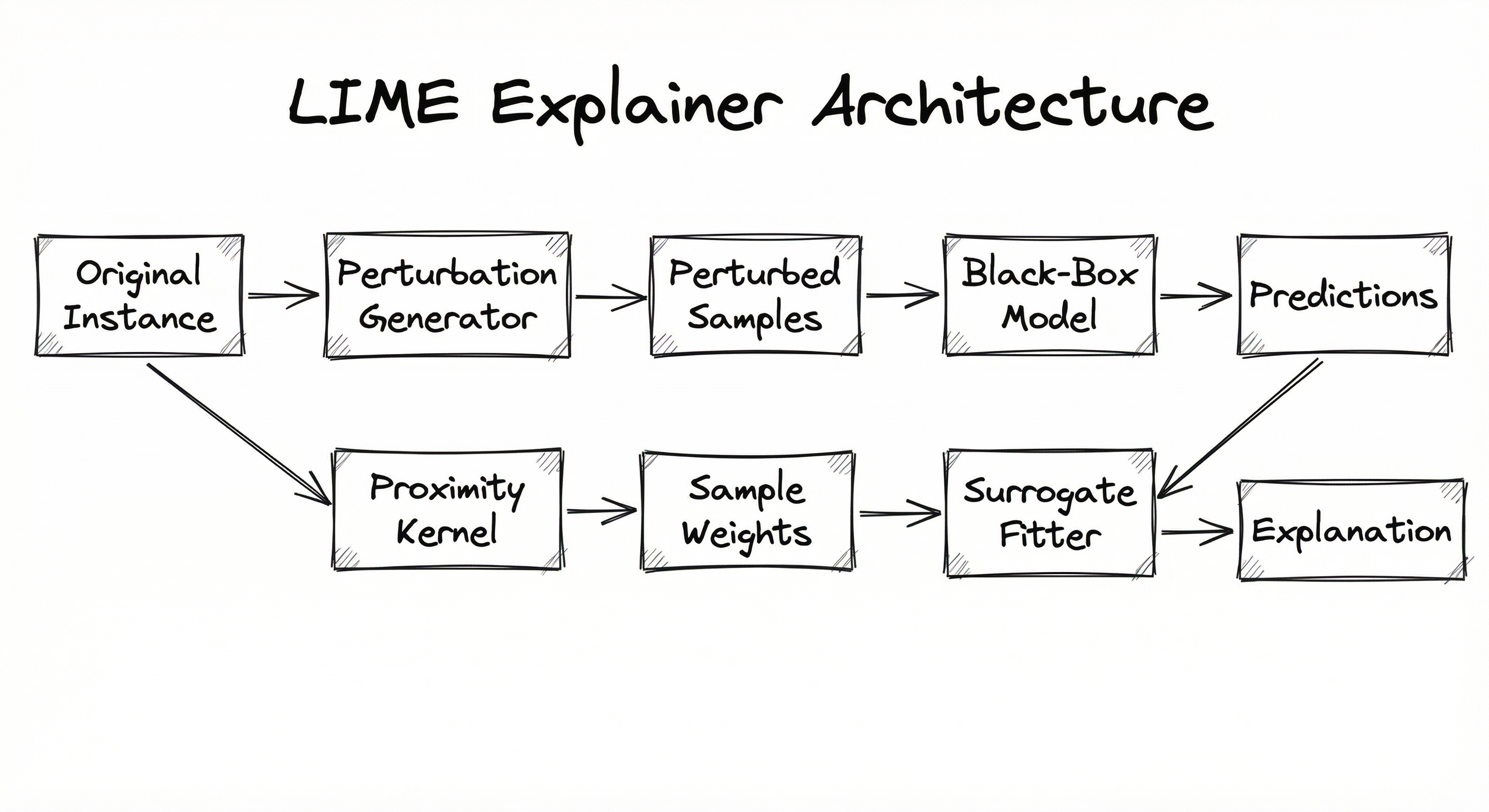
LIME's architecture is a pipeline of five stages: input preparation, perturbation generation, black-box querying, proximity weighting, and surrogate model fitting. The architecture is deliberately modular -- each stage can be customized for different data types (tabular, text, image) without changing the overall flow.
The perturbation generator is the most data-type-specific component. For tabular data, it samples from marginal feature distributions. For text, it randomly removes tokens. For images, it segments the image into superpixels (using algorithms like quickshift or SLIC) and then randomly masks subsets of superpixels.
The surrogate model fitter is typically a weighted Lasso or Ridge regression, but it can be replaced with any interpretable model class (decision stumps, short rule lists, etc.). The choice affects the form of the explanation: linear coefficients vs. if-then rules.
Key Components
Perturbation Generator
Creates perturbed versions of the input instance. For tabular data, it samples feature values from the training distribution (mean and standard deviation per feature). For text, it randomly drops words from the original document. For images, it first segments the image into superpixels (contiguous regions of similar pixels) using quickshift or SLIC, then randomly masks subsets of these superpixels. The interpretable representation (a binary vector indicating which features/words/superpixels are present) is generated simultaneously.
Black-Box Oracle
The black-box model treated as a callable prediction function. LIME only requires predict() (for classification) or predict_proba() access -- no gradients, no internal weights, no architecture knowledge. This is what makes LIME truly model-agnostic. The oracle is queried times per explanation, making inference cost the dominant expense.
Proximity Kernel
Computes a weight for each perturbed sample based on its distance from the original instance . Uses an exponential (RBF) kernel with configurable kernel width . Closer perturbations receive higher weights, enforcing locality. The kernel width is the single most important hyperparameter in LIME and directly controls the fidelity-coverage tradeoff.
Surrogate Model Fitter
Fits a weighted interpretable model (typically sparse linear regression via Lasso) on the dataset of (perturbed interpretable representations, black-box predictions, proximity weights). The resulting model coefficients serve as feature importance scores. The sparsity constraint (maximum number of non-zero features in the explanation) is user-configurable and controls explanation complexity.
Explanation Renderer
Formats the surrogate model's output into human-readable explanations. For tabular data: a ranked list of feature contributions with signs and magnitudes. For text: highlighted words with positive/negative color coding. For images: a heatmap overlay showing which superpixels contributed most to the prediction. Integrates with visualization libraries like matplotlib.
Data Flow
Step 1: Prepare. The original instance is converted into an interpretable representation (binary vector). For tabular data, is all 1s (all features present). For text, is all 1s (all words present). For images, is all 1s (all superpixels visible).
Step 2: Perturb. The perturbation generator creates binary vectors by randomly flipping bits in . Each is then mapped back to the original feature space to create a concrete perturbed instance .
Step 3: Query. Each perturbed instance is fed through the black-box model to obtain predictions . This is the most expensive step.
Step 4: Weight. The proximity kernel computes for each perturbed sample, assigning higher weights to samples closer to the original instance.
Step 5: Fit. A weighted Lasso regression is fitted: . The non-zero coefficients and their signs indicate which features pushed the prediction up or down.
Step 6: Render. The explanation is formatted for the target audience -- engineers get raw coefficients, business stakeholders get natural-language summaries, compliance teams get structured audit logs.
A directed pipeline: Original Instance feeds into the Perturbation Generator, which produces Perturbed Samples. These flow into the Black-Box Model to generate Predictions. The Original Instance also feeds the Proximity Kernel to produce Sample Weights. Predictions, Perturbed Samples, and Sample Weights all converge into the Weighted Surrogate Fitter, which outputs the final Explanation (Feature Importances).
How to Implement
Getting Started with LIME
The lime Python library (maintained by Marco Tulio Ribeiro) provides production-ready implementations for tabular, text, and image data. It is the canonical implementation and integrates seamlessly with scikit-learn, TensorFlow, Keras, PyTorch, and XGBoost. Installation is straightforward: pip install lime.
The library exposes three main explainer classes: LimeTabularExplainer for structured/tabular data, LimeTextExplainer for NLP tasks, and LimeImageExplainer for computer vision. Each class handles the data-type-specific perturbation logic internally, so you only need to provide the model's prediction function and the instance to explain.
Production Considerations
In production, LIME explanations are typically generated offline or asynchronously rather than in the critical path of real-time inference. The reason is cost: each explanation requires (default 5000) forward passes through the model. For a model with 10ms inference latency, that is 50 seconds per explanation.
For offline auditing and batch explanation generation, this is perfectly acceptable. For near-real-time use cases (e.g., explaining a loan rejection to a customer within seconds), teams typically pre-compute explanations for common prediction buckets or use a smaller (500-1000) with acceptance of slightly noisier explanations.
Cost Note: On AWS
ml.m5.xlarge(~0.50-0.526/hr, ~INR 44/hr), the same 10,000 explanations might take 8-12 hours due to higher per-inference cost, totaling ~$4-6 (~INR 336-504). Budget accordingly.
import numpy as np
import pandas as pd
from sklearn.ensemble import GradientBoostingClassifier
from sklearn.model_selection import train_test_split
from lime.lime_tabular import LimeTabularExplainer

# Load and prepare data (example: loan default dataset)
df = pd.read_csv("loan_data.csv")
feature_names = ["income", "loan_amount", "credit_score", "employment_years",
                 "debt_to_income", "num_open_accounts", "delinquencies"]
X = df[feature_names].values
y = df["default"].values

X_train, X_test, y_train, y_test = train_test_split(X, y, test_size=0.2, random_state=42)

# Train a black-box model
model = GradientBoostingClassifier(n_estimators=200, max_depth=5, random_state=42)
model.fit(X_train, y_train)

# Create LIME explainer
explainer = LimeTabularExplainer(
    training_data=X_train,
    feature_names=feature_names,
    class_names=["no_default", "default"],
    mode="classification",
    discretize_continuous=True,     # bin continuous features for cleaner explanations
    kernel_width=None,              # None uses default: sqrt(num_features) * 0.75
    sample_around_instance=True,    # perturb around the instance, not globally
    random_state=42                 # for reproducibility
)

# Explain a single prediction
instance = X_test[0]
explanation = explainer.explain_instance(
    data_row=instance,
    predict_fn=model.predict_proba,
    num_features=5,         # top 5 features in explanation
    num_samples=1000        # number of perturbations
)

# Access explanation data programmatically
print("Prediction probabilities:", model.predict_proba([instance])[0])
print("\nTop feature contributions:")
for feature, weight in explanation.as_list():
    direction = "increases" if weight > 0 else "decreases"
    print(f"  {feature}: {weight:+.4f} ({direction} default probability)")

# Local fidelity score (R-squared of the surrogate model)
print(f"\nLocal model R-squared: {explanation.score:.4f}")

# Save explanation as HTML
explanation.save_to_file("lime_explanation.html")
This example demonstrates LIME for a loan default prediction model -- a common use case in Indian fintech. The LimeTabularExplainer is initialized with training data (needed to compute feature statistics for perturbation), feature names, and class labels. The explain_instance method generates perturbations, queries the model, fits the surrogate, and returns a structured explanation. Key parameters: num_features controls explanation sparsity (how many features appear), num_samples controls the number of perturbations (more = stabler but slower), and kernel_width controls locality. The score attribute reports the surrogate model's -- a direct measure of local fidelity.
from lime.lime_text import LimeTextExplainer
from sklearn.pipeline import make_pipeline
from sklearn.feature_extraction.text import TfidfVectorizer
from sklearn.linear_model import LogisticRegression

# Train a text classifier (example: product review sentiment)
train_texts = [
    "This phone has an amazing camera and great battery life",
    "Terrible product, stopped working after one week",
    "Decent value for money, delivery was fast on Flipkart",
    "Worst purchase ever, screen cracked immediately",
    # ... more training data
]
train_labels = [1, 0, 1, 0]  # 1=positive, 0=negative

pipeline = make_pipeline(
    TfidfVectorizer(max_features=5000),
    LogisticRegression(C=1.0)
)
pipeline.fit(train_texts, train_labels)

# Create LIME text explainer
text_explainer = LimeTextExplainer(
    class_names=["negative", "positive"],
    split_expression=r'\W+',    # tokenize on non-word characters
    bow=True,                     # use bag-of-words representation
    random_state=42
)

# Explain a specific review
review = "The camera quality is outstanding but the battery drains too quickly"
text_explanation = text_explainer.explain_instance(
    text_instance=review,
    classifier_fn=pipeline.predict_proba,
    num_features=6,
    num_samples=2000
)

# Print word-level contributions
print(f"Predicted class: {'positive' if pipeline.predict([review])[0] == 1 else 'negative'}")
print(f"Prediction confidence: {pipeline.predict_proba([review])[0]}")
print("\nWord contributions:")
for word, weight in text_explanation.as_list():
    print(f"  '{word}': {weight:+.4f}")

# Generate HTML with highlighted words
text_explanation.save_to_file("text_explanation.html")
LIME for text works by randomly removing words and observing how the model's prediction changes. Words that significantly alter the prediction when removed receive high importance weights. In this Flipkart product review example, you would expect words like "outstanding" to have positive weight and "drains" to have negative weight. The bow=True parameter uses bag-of-words representation where each word is treated independently -- this is the default and works well for most text classifiers. Set bow=False if word order matters for your model.
import numpy as np
from lime import lime_image
from skimage.segmentation import mark_boundaries
import matplotlib.pyplot as plt
from tensorflow.keras.applications import ResNet50
from tensorflow.keras.applications.resnet50 import preprocess_input, decode_predictions
from tensorflow.keras.preprocessing import image as keras_image

# Load pre-trained model
model = ResNet50(weights="imagenet")

def predict_fn(images):
    """Wrapper to match LIME's expected interface."""
    preprocessed = preprocess_input(images.copy())
    return model.predict(preprocessed)

# Load and prepare image
img_path = "chest_xray.jpg"
img = keras_image.load_img(img_path, target_size=(224, 224))
img_array = np.array(img)

# Create LIME image explainer
image_explainer = lime_image.LimeImageExplainer(random_state=42)

# Generate explanation
image_explanation = image_explainer.explain_instance(
    image=img_array.astype("double"),
    classifier_fn=predict_fn,
    top_labels=3,
    hide_color=0,            # black out masked superpixels
    num_samples=1000,
    segmentation_fn=None     # uses quickshift by default
)

# Visualize: show superpixels that support the top prediction
top_label = image_explanation.top_labels[0]
temp, mask = image_explanation.get_image_and_mask(
    label=top_label,
    positive_only=True,      # only show supporting regions
    num_features=5,          # top 5 superpixels
    hide_rest=True           # hide non-contributing regions
)

fig, axes = plt.subplots(1, 3, figsize=(15, 5))
axes[0].imshow(img_array)
axes[0].set_title("Original Image")
axes[1].imshow(mark_boundaries(temp / 255.0, mask))
axes[1].set_title(f"LIME Explanation (top class)")

# Show both positive and negative contributions
temp2, mask2 = image_explanation.get_image_and_mask(
    label=top_label,
    positive_only=False,
    num_features=10,
    hide_rest=False
)
axes[2].imshow(mark_boundaries(temp2 / 255.0, mask2))
axes[2].set_title("Positive (green) & Negative (red)")
plt.tight_layout()
plt.savefig("lime_image_explanation.png", dpi=150)
plt.show()
LIME for images works by first segmenting the image into superpixels (contiguous regions of similar pixels), then randomly masking subsets of superpixels and observing how the prediction changes. Superpixels that, when masked, cause the prediction confidence to drop significantly are deemed important. This is particularly valuable in medical imaging (e.g., chest X-ray analysis at hospitals like AIIMS or Apollo), where clinicians need to see which regions drove the model's diagnosis. The hide_color=0 parameter blacks out masked regions; setting it to the mean pixel value often produces more realistic perturbations.
import numpy as np
from lime.lime_tabular import LimeTabularExplainer
from collections import defaultdict

def generate_stable_explanation(
    explainer: LimeTabularExplainer,
    instance: np.ndarray,
    predict_fn,
    num_features: int = 5,
    num_samples: int = 2000,
    n_repeats: int = 5,
    stability_threshold: float = 0.8
):
    """
    Generate a LIME explanation with stability assessment.
    Runs LIME multiple times and checks if feature rankings are consistent.
    """
    all_explanations = []
    feature_rank_counts = defaultdict(list)

    for i in range(n_repeats):
        exp = explainer.explain_instance(
            data_row=instance,
            predict_fn=predict_fn,
            num_features=num_features,
            num_samples=num_samples
        )
        features_in_explanation = [feat for feat, _ in exp.as_list()]
        all_explanations.append(exp)

        for rank, feat in enumerate(features_in_explanation):
            feature_rank_counts[feat].append(rank)

    # Compute stability: fraction of runs where the top feature set is identical
    top_feature_sets = [
        frozenset(feat for feat, _ in exp.as_list())
        for exp in all_explanations
    ]
    most_common_set = max(set(top_feature_sets), key=top_feature_sets.count)
    stability_score = top_feature_sets.count(most_common_set) / n_repeats

    # Compute average R-squared (local fidelity)
    avg_r2 = np.mean([exp.score for exp in all_explanations])

    # Use the explanation from the run with highest R-squared
    best_explanation = max(all_explanations, key=lambda e: e.score)

    result = {
        "explanation": best_explanation,
        "stability_score": stability_score,
        "is_stable": stability_score >= stability_threshold,
        "avg_local_fidelity": avg_r2,
        "feature_consistency": {
            feat: len(ranks) / n_repeats
            for feat, ranks in feature_rank_counts.items()
        }
    }

    if not result["is_stable"]:
        print(f"WARNING: Explanation stability ({stability_score:.2f}) below "
              f"threshold ({stability_threshold}). Consider increasing num_samples "
              f"or adjusting kernel_width.")

    return result

# Usage
result = generate_stable_explanation(
    explainer=explainer,
    instance=X_test[0],
    predict_fn=model.predict_proba,
    num_features=5,
    num_samples=2000,
    n_repeats=5
)

print(f"Stability score: {result['stability_score']:.2f}")
print(f"Average local fidelity (R^2): {result['avg_local_fidelity']:.4f}")
print(f"Stable: {result['is_stable']}")
print(f"Feature consistency: {result['feature_consistency']}")
One of LIME's well-known weaknesses is instability: running LIME multiple times on the same instance can produce different explanations due to the random perturbation sampling. This wrapper runs LIME n_repeats times, measures the consistency of the top feature set across runs (stability score), and returns the explanation with the highest local fidelity (). If stability is below the threshold, it warns the user to increase num_samples or adjust kernel_width. This pattern is essential for production deployments where explanation reliability matters -- especially in regulated contexts like credit scoring at Indian NBFCs.
# LIME configuration for production audit pipeline (YAML)
explainer:
  type: tabular
  training_data_path: "s3://ml-data/training_features.parquet"
  feature_names_path: "s3://ml-config/feature_names.json"
  class_names: ["approved", "rejected"]
  mode: "classification"
  discretize_continuous: true
  kernel_width: 3.0        # tuned for this dataset; default was 2.6
  random_state: 42

explanation:
  num_features: 7          # top 7 features per explanation
  num_samples: 3000        # balance between stability and cost
  n_repeats: 3             # stability check: run 3 times
  stability_threshold: 0.8 # warn if <80% consistent

output:
  format: "json"           # structured for downstream consumption
  include_r_squared: true  # local fidelity score
  storage: "azure-table"   # persist explanations for audit trail
  retention_days: 365      # regulatory retention requirement
Common Implementation Mistakes
- ●
Using default kernel_width without validation: The default kernel width (
0.75 * sqrt(num_features)) is a reasonable heuristic but can be wildly inappropriate for specific datasets. Always check the surrogate model's score -- if it is below 0.5, the local approximation is poor and you should adjust the kernel width or increasenum_samples. - ●
Ignoring LIME's instability: Running LIME once and treating the explanation as ground truth. Due to random perturbation sampling, two runs on the same instance can produce different top features. Always run multiple repetitions and check consistency, especially for high-stakes decisions like loan approvals or medical diagnoses.
- ●
Explaining predictions without checking model accuracy first: LIME explains what the model does, not what it should do. If the model itself is wrong (low accuracy on the test set), LIME will faithfully explain the wrong prediction. Always validate model performance before investing in explainability.
- ●
Setting num_samples too low for high-dimensional data: For tabular data with 50+ features or images with hundreds of superpixels, 500 perturbations are insufficient for a stable surrogate fit. Use at least 2000-5000 samples for moderate-dimensional data and 5000-10000 for high-dimensional cases.
- ●
Treating LIME feature importances as causal: LIME shows correlational contributions to the prediction, not causal effects. A feature having high LIME weight means removing it changes the prediction -- it does not mean that feature caused the outcome in the real world. This distinction is critical for compliance reports.
- ●
Using LIME for global model understanding: LIME is designed for individual predictions. Aggregating LIME explanations across many instances to infer global feature importance is possible but statistically unreliable and much slower than using SHAP's global summary plots. Use the right tool for the right scope.
When Should You Use This?
Use When
You need per-prediction explanations for individual instances, not just global feature importance -- e.g., explaining why a specific loan was rejected at Bajaj Finance or why a specific transaction was flagged as fraud at PhonePe
Your model is a black box (deep neural network, ensemble, or third-party API) and you cannot access internal weights or gradients
You need a model-agnostic method that works across scikit-learn, TensorFlow, PyTorch, XGBoost, and even external API endpoints without any code changes
Your use case involves tabular, text, or image data -- LIME has native, well-tested support for all three modalities
You are working in a regulated industry (banking under RBI FREE-AI, insurance under IRDAI, healthcare under MCI guidelines) where per-decision explanations are mandated
You need human-readable explanations that non-technical stakeholders (compliance officers, doctors, loan officers) can understand
Explanation generation can happen offline or asynchronously -- you do not need sub-second explanation latency
Avoid When
You need real-time explanations in the critical inference path (LIME typically takes 5-50 seconds per explanation depending on model complexity and num_samples). Consider gradient-based methods (Integrated Gradients, GradCAM) for real-time needs.
You need global model interpretability (understanding which features matter across the entire dataset). SHAP's global summary plots or permutation importance are better suited.
Your model is inherently interpretable (logistic regression, small decision tree, GAM). There is no point in fitting a surrogate model to explain a model that is already interpretable -- just read the coefficients directly.
Explanation stability is critical and you cannot afford to run multiple repetitions. LIME's stochastic nature means a single run may not be reproducible. Consider Anchors or SHAP TreeExplainer for deterministic explanations.
You are explaining a model with very high inference cost (e.g., a large language model at 50 (~INR 4,200) in API calls alone.
Feature interactions are the primary phenomenon you need to explain. LIME's linear surrogate model cannot capture interaction effects. Use SHAP interaction values or partial dependence plots instead.
Key Tradeoffs
The Fidelity-Interpretability Spectrum
LIME's central tradeoff is between local fidelity (how accurately the surrogate mimics the black box near the instance) and interpretability (how simple and understandable the explanation is). Increasing num_features in the explanation improves fidelity but makes the explanation harder for humans to digest. In practice, 5-10 features per explanation is the sweet spot for tabular data.
| Parameter | Increase Effect | Decrease Effect |
|---|---|---|
num_samples | Stabler explanations, higher cost | Noisier explanations, lower cost |
kernel_width | Broader locality, smoother explanations | Tighter locality, more instance-specific |
num_features | Higher fidelity (), harder to read | Lower fidelity, easier to read |
n_repeats (stability) | More confidence in explanation | Faster but less reliable |
LIME vs. SHAP: The Practical Tradeoff
LIME is faster for single explanations (especially for non-tree models) but less stable. SHAP (particularly TreeSHAP) is exact and deterministic for tree-based models but computationally expensive for deep learning models. For a gradient-boosted model at Zerodha's risk engine processing 100K predictions/day:
- LIME: ~10 seconds/explanation, stochastic, ~INR 84/10K explanations on AWS
- SHAP TreeExplainer: ~0.1 seconds/explanation, deterministic, ~INR 1/10K explanations
- SHAP KernelSHAP: ~30 seconds/explanation, approximately deterministic, ~INR 252/10K explanations
For tree models, SHAP wins on every axis. LIME's advantage emerges with non-tree models (neural networks, SVMs, black-box APIs) where TreeSHAP is unavailable.
Rule of Thumb: Use SHAP TreeExplainer for tree-based models. Use LIME for everything else, or when you need a quick, model-agnostic baseline.
Alternatives & Comparisons
SHAP provides theoretically grounded feature attributions based on Shapley values from cooperative game theory. Unlike LIME, SHAP satisfies desirable axioms (local accuracy, missingness, consistency) and offers both local and global explanations. TreeSHAP is exact and deterministic for tree models. Choose SHAP when you need theoretical guarantees, global+local explanations, or are working with tree-based models. Choose LIME when you need model-agnostic explanations for neural networks or API-based models, or when SHAP's computational cost is prohibitive.
Bias detectors identify systematic disparities in model predictions across protected groups (gender, caste, religion, age). LIME explains individual predictions; bias detectors audit population-level fairness. They are complementary: use LIME to explain why a specific decision was made, and bias detectors to check whether decisions are systematically unfair across groups. In practice, LIME explanations can reveal biased features (e.g., zip code as a proxy for caste) that bias detectors flag at the aggregate level.
Fairness checkers evaluate whether a model meets specific fairness criteria (demographic parity, equalized odds, calibration across groups). LIME does not measure fairness -- it explains predictions. However, LIME can be used as a diagnostic tool when a fairness checker flags a violation: you can LIME-explain predictions for different subgroups to understand which features drive the disparity. Use fairness checkers for the 'what' (is it fair?) and LIME for the 'why' (why is it unfair?).
Anchors, also by Ribeiro et al. (AAAI 2018), generate if-then rule-based explanations with probabilistic precision guarantees. While LIME produces feature weights (continuous), Anchors produce sufficient conditions (binary rules). Anchors are deterministic and more stable than LIME, but less flexible -- they work best for classification and struggle with regression. Choose Anchors when you need rule-based explanations with coverage guarantees; choose LIME when you need continuous feature importance scores.
Pros, Cons & Tradeoffs
Advantages
Truly model-agnostic: Works with any model that has a
predictorpredict_probafunction -- scikit-learn, TensorFlow, PyTorch, XGBoost, LightGBM, CatBoost, cloud APIs, and even ensemble stacks. No architecture-specific code needed.Multi-modal support: Native implementations for tabular data, text (bag-of-words perturbation), and images (superpixel masking). One framework covers the three most common ML data types in production.
Human-readable explanations: Produces ranked feature contributions with positive/negative signs and magnitudes that non-technical stakeholders (loan officers, doctors, compliance teams) can understand without ML knowledge.
Mature ecosystem and tooling: The
limePython library has 11K+ GitHub stars, extensive documentation, and integrates with InterpretML, Alibi, and MLflow. Battle-tested since 2016 with broad community support.Regulatory acceptance: Explicitly named in India's RBI FREE-AI framework (2025) and the EU AI Act guidance as an acceptable explanation method. Using LIME provides tangible compliance evidence during audits.
Lightweight infrastructure requirements: No GPU required for generating explanations (the perturbation and surrogate fitting are CPU-only). The cost is entirely in the forward passes through the black-box model.
Configurable explanation complexity: The
num_featuresparameter lets you control how many features appear in the explanation -- 3 features for a customer-facing summary, 10 features for an internal audit report.
Disadvantages
Instability across runs: Due to random perturbation sampling, LIME can produce different explanations for the same instance on different runs. This is a well-documented limitation that requires mitigation (multiple runs, stability checks, or variants like S-LIME/BayLIME).
Computational cost scales with model inference: Each explanation requires (500-5000) forward passes through the black-box model. For expensive models (large neural networks, LLM APIs), this makes LIME prohibitively slow and expensive for real-time use.
Kernel width sensitivity: The explanation quality depends heavily on the kernel width parameter, which controls the locality of the approximation. There is no universally optimal value -- it must be tuned per dataset, and poor choices can produce misleading explanations.
Linear surrogate cannot capture interactions: The default linear surrogate model assumes features contribute independently. When the black-box model relies on feature interactions (e.g., income x debt_to_income), LIME's linear approximation will miss or misattribute these effects.
No theoretical guarantees: Unlike SHAP (which satisfies Shapley axioms), LIME does not guarantee properties like local accuracy or consistency. The quality of the explanation depends entirely on the quality of the local approximation, which is hard to verify without ground truth.
Perturbation distribution can be unrealistic: For tabular data, LIME perturbs features independently from their marginal distributions, which can generate out-of-distribution samples (e.g., a 25-year-old with 30 years of work experience). These unrealistic samples can distort the surrogate model's fit.
Failure Modes & Debugging
Explanation instability (non-reproducibility)
Cause
Random perturbation sampling produces different neighbor sets on each run. With a limited num_samples (e.g., 500), the variance in the sampled neighborhood can be high, leading to different feature rankings across runs.
Symptoms
Running LIME twice on the same instance yields different top features or different signs on feature weights. A compliance team reviewing explanations finds contradictory reasons for the same decision. Users lose trust in the explanation system.
Mitigation
- Increase
num_samplesto 2000-5000 to reduce sampling variance. 2) Setrandom_statefor reproducibility in auditing contexts. 3) Run multiple repetitions and report consensus features (see the stability wrapper code example above). 4) Consider S-LIME or BayLIME for inherently more stable explanations.
Poor local fidelity (low surrogate R-squared)
Cause
The linear surrogate model cannot adequately approximate the black box's behavior in the local neighborhood. This happens when: (a) the kernel width is too large (the neighborhood includes regions where the model is highly non-linear), (b) the black box has strong feature interactions that a linear model cannot capture, or (c) num_features is set too low, forcing the surrogate to use too few features.
Symptoms
The explanation.score () is below 0.3-0.5. Feature importances feel random or counterintuitive. Explanations do not match domain expert expectations even when the model is known to be well-calibrated.
Mitigation
- Decrease kernel width to focus on a tighter neighborhood. 2) Increase
num_featuresto allow the surrogate more expressive power. 3) For highly non-linear regions, consider switching to Anchors (rule-based) or SHAP (which handles interactions better). 4) Always report alongside the explanation as a confidence indicator.
Out-of-distribution perturbations (tabular data)
Cause
LIME perturbs each feature independently from its marginal distribution, ignoring feature correlations. This generates synthetic instances that could never occur in reality (e.g., a person with income = INR 2 lakh/year but a home loan of INR 5 crore). The black-box model's behavior on these unrealistic inputs may be undefined or erratic.
Symptoms
Surrogate model learns from model behavior on unrealistic inputs, producing explanations that do not reflect how the model treats realistic perturbations. Feature importances may be inflated for correlated features.
Mitigation
- Use
sample_around_instance=True(enabled by default in recent versions) to perturb around the instance rather than from the global distribution. 2) Implement custom perturbation functions that respect feature correlations (e.g., using a multivariate Gaussian fitted to the training data). 3) Post-filter perturbations to remove obviously impossible combinations.
Superpixel segmentation failure (images)
Cause
The default quickshift segmentation algorithm may produce superpixels that do not align with semantically meaningful regions of the image. For medical images (X-rays, MRIs), the default parameters often create either too-fine or too-coarse segmentations.
Symptoms
Image explanations highlight seemingly arbitrary regions that do not correspond to any clinically meaningful anatomy. Superpixels split important structures (e.g., a tumor) across multiple segments, diluting their importance.
Mitigation
- Tune quickshift parameters (
kernel_size,max_dist,ratio) for your image domain. 2) Use a custom segmentation function (e.g., Felzenszwalb, SLIC, or a domain-specific segmenter). 3) For medical imaging, consider using anatomical region priors as the segmentation basis.
Misleading explanations under distribution shift
Cause
LIME explains the model's behavior at a specific input point. If the production data distribution has shifted since the model was trained, the model may be making predictions in an extrapolation regime where its behavior is unreliable. LIME will faithfully explain the unreliable prediction, making it look legitimate.
Symptoms
Explanations appear plausible but the underlying prediction is wrong due to distribution shift. Stakeholders trust the explanation and act on an incorrect prediction. This is particularly dangerous in dynamic environments (e.g., credit scoring during an economic downturn).
Mitigation
- Always pair LIME with model monitoring (distribution shift detection, prediction confidence tracking). 2) Flag explanations for instances where the model's confidence is low or the instance is far from the training distribution. 3) Never present LIME explanations without also showing the model's confidence score.
Kernel width misconfiguration
Cause
The kernel width is set too large (explanations average over too broad a region, losing locality) or too small (explanations are hypersensitive to noise in the immediate neighborhood). The default heuristic (0.75 * sqrt(num_features)) is not universally appropriate.
Symptoms
Too large: explanations are too similar across very different instances (LIME is explaining the global model, not the local prediction). Too small: explanations are noisy and unstable, changing dramatically with tiny input perturbations.
Mitigation
- Evaluate scores across a representative sample of instances at different kernel widths. 2) Choose the kernel width that maximizes the median while keeping explanation stability above your threshold. 3) Consider adaptive kernel width selection based on local data density.
Placement in an ML System
Where LIME Sits in the ML System
In a production ML system, LIME operates in the post-prediction audit layer -- after the model has made a prediction but before the decision is communicated to the end user or acted upon by a downstream system.
For synchronous use cases (rare, due to latency), LIME sits between the inference service and the response formatter. The prediction is made, LIME generates an explanation, and both are returned together. This is feasible only for lightweight models with fast inference (e.g., a scikit-learn model on tabular data).
For asynchronous use cases (the common pattern), LIME runs as a background job. The prediction is served immediately, and LIME explanations are generated in a batch pipeline and stored for later retrieval. When a compliance officer, loan officer, or customer requests an explanation, it is fetched from the explanation store (Azure Table Storage, PostgreSQL, etc.).
LIME interacts with the bias detector and fairness checker downstream: these tools can consume LIME explanations to understand why the model exhibits the biases or unfairness they detect. For example, if a fairness checker flags that loan rejection rates are higher for a protected group, LIME explanations for rejected instances from that group can reveal which features are driving the disparity.
Architecture Pattern: In Indian fintech companies complying with RBI FREE-AI, the typical setup is: Prediction Service -> Explanation Queue (SQS/Kafka) -> LIME Worker Pool -> Explanation Store (Azure Table / DynamoDB) -> Compliance Dashboard.
Pipeline Stage
Post-Prediction / Model Audit
Upstream
- model-serving
- inference-pipeline
- prediction-store
Downstream
- bias-detector
- fairness-checker
- compliance-dashboard
- human-review-queue
Scaling Bottlenecks
The primary bottleneck is the number of forward passes through the black-box model. Each explanation requires calls to predict() or predict_proba(). At scale:
- 10K explanations/day with perturbations = 20 million model inferences/day just for explainability. If each inference takes 10ms, that is ~55 hours of sequential compute -- you need parallelism.
- Cost on AWS: For a scikit-learn model on
ml.m5.xlarge(~INR 19/hr), 10K explanations/day costs ~INR 1,050/day (~INR 31,500/month). For a TensorFlow model onml.g4dn.xlarge(~INR 44/hr), it scales to ~INR 2,400/day (~INR 72,000/month, ~$860/month).
Scaling strategies: (1) Batch perturbations and use vectorized model inference. (2) Cache explanations for common prediction patterns. (3) Use a distilled student model for LIME queries instead of the full production model. (4) Reduce for non-critical explanations and reserve high- for audit-flagged instances.
Production Case Studies
JPMorgan Chase uses LIME alongside SHAP to explain credit risk model predictions for regulatory compliance. Their Explainable AI (XAI) program generates per-decision explanations for loan underwriting models, enabling loan officers to provide clear reasons for approval or denial. The explanations are stored in an audit trail that regulators can review during examinations.
Improved regulatory compliance with the Equal Credit Opportunity Act (ECOA) requirement to provide specific reasons for credit denials. Reduced model review cycle time by 40% by giving risk analysts direct visibility into feature contributions.
Agarwal et al. document Apollo Hospitals' implementation of AI-based healthcare including robotic surgery and AI systems. The use of AI allows medical practitioners to provide more personalized health care, increases physician efficiency by removing repetitive tasks, and facilitates a shift toward prevention of serious illnesses through early detection.
Apollo Hospitals deployed AI across radiology for TB and cancer detection (winning grants from Bill & Melinda Gates Foundation), with Google Health partnership enabling accurate chest X-ray interpretation for early TB signs.
Lendingkart, an Indian MSME lending platform, uses LIME to explain their credit scoring models for small business loans. When a loan application is processed, LIME generates feature-level explanations showing which factors (GST filing history, bank statement patterns, business vintage, industry risk score) most influenced the credit decision. These explanations are made available to both internal underwriters and the applicants themselves.
Achieved compliance with RBI's fair lending guidelines by providing specific, per-application reasons for credit decisions. Customer complaints about opaque rejections decreased by approximately 25%, and loan officers reported faster decision-making with LIME-assisted reviews.
Hugging Face integrated LIME-based explanations into their model evaluation pipeline, enabling users to understand why transformer-based text classifiers make specific predictions. The integration allows model developers to debug misclassifications by visualizing which tokens drove incorrect predictions, facilitating faster iteration on model training and data quality.
Model debugging time for text classification tasks reduced by an estimated 30-50% when developers used LIME explanations to trace misclassifications back to training data issues or tokenization artifacts.
Tooling & Ecosystem
The original LIME library by Marco Tulio Ribeiro. Provides LimeTabularExplainer, LimeTextExplainer, and LimeImageExplainer. Integrates with scikit-learn, TensorFlow, Keras, PyTorch, and XGBoost. The canonical, most widely used implementation with 11K+ GitHub stars.
Microsoft's unified framework for interpretable ML. Includes LIME (via LimeTabular) alongside EBM (Explainable Boosting Machine), SHAP, and other explainability methods. Provides a consistent API and interactive dashboards for comparing explanation methods side by side.
Seldon's ML model inspection and interpretation library. Includes LIME implementations plus Anchors, counterfactual explanations, and contrastive explanations. Designed for production deployment with Seldon Core. Strong integration with Kubernetes-based ML serving.
Descriptive mAchine Learning EXplanations. Wraps LIME and other explanation methods (SHAP, Break Down, Ceteris Paribus) in a unified interface. Excellent visualization capabilities and the companion fairmodels package for fairness analysis. Particularly popular in the R community.
PyTorch's official model interpretability library. While it focuses on gradient-based methods (Integrated Gradients, DeepLIFT, GradCAM), it includes LIME as one of its attribution methods. Best for PyTorch-native workflows where you want both gradient and perturbation-based explanations.
Bayesian extension of LIME that incorporates prior knowledge and Bayesian reasoning to improve explanation stability and robustness to kernel width settings. Addresses LIME's instability problem by replacing the frequentist Lasso with Bayesian linear regression.
Salesforce's comprehensive XAI library supporting tabular, text, image, and time-series data. Includes LIME alongside 20+ other explanation methods (SHAP, Integrated Gradients, counterfactuals). Provides a unified API and an interactive dashboard for comparing explanations.
Research & References
Ribeiro, Singh & Guestrin (2016)KDD 2016
The foundational LIME paper. Introduced the concept of local interpretable surrogate models, the perturbation-based explanation framework, and SP-LIME for selecting representative explanations. Over 11,000 citations -- one of the most influential XAI papers ever published.
Ribeiro, Singh & Guestrin (2018)AAAI 2018
The follow-up to LIME by the same authors. Introduces Anchor explanations: if-then rules with probabilistic precision guarantees. Addresses LIME's instability and the difficulty of choosing kernel width by producing deterministic, coverage-bounded rules.
Lundberg & Lee (2017)NeurIPS 2017
Introduced SHAP, which unifies LIME and several other explanation methods under a Shapley value framework. Shows that LIME is a special case of the SHAP framework with specific kernel weights. Essential reading for understanding LIME's theoretical position.
Zhou, Hooker & Wang (2021)arXiv preprint
Proposes S-LIME, which uses a hypothesis testing framework based on the central limit theorem to determine the minimum number of perturbation samples needed for a stable LIME explanation. Provides principled guidance on the num_samples parameter.
Visani, Bagli, Berber & Guidotti (2020)Journal of the Operational Research Society
Formally quantifies LIME's instability problem and proposes statistical indices to measure explanation reliability. Demonstrates that LIME explanations can vary significantly across runs and provides metrics to assess when explanations are trustworthy.
Salih, Galazzo, Raisi-Estabragh et al. (2025)Advanced Intelligent Systems (Wiley)
Comprehensive 2024-2025 perspective comparing SHAP and LIME across healthcare, finance, and NLP applications. Analyzes strengths, limitations, and practical guidance for choosing between the two methods in production settings.
Zafar, Khan & Iqbal (2025)arXiv preprint
A 2025 survey cataloging LIME variants (S-LIME, BayLIME, US-LIME, DLIME, LS-LIME) and analyzing their relative strengths. Provides a decision framework for selecting the appropriate LIME variant based on the use case, data type, and stability requirements.
Interview & Evaluation Perspective
Common Interview Questions
- ●
Explain how LIME works. Walk me through generating an explanation for a single prediction.
- ●
What is the fidelity-interpretability tradeoff in LIME, and how do you manage it in practice?
- ●
LIME is known to be unstable -- what does that mean, and how would you mitigate it in a production system?
- ●
How does LIME differ from SHAP? When would you choose one over the other?
- ●
You are building a credit scoring model for an Indian NBFC that must comply with RBI explainability guidelines. How would you integrate LIME?
- ●
What happens if you set the kernel width too large or too small in LIME?
- ●
How does LIME handle image data differently from tabular data?
- ●
Can LIME explanations be used as evidence of non-discrimination in a regulatory audit?
Key Points to Mention
- ●
LIME fits a local, interpretable surrogate (sparse linear model) around a single prediction by perturbing the input and observing how the black-box model's output changes. The surrogate's coefficients are the explanation.
- ●
The kernel width controls locality: too small = noisy/unstable, too large = loses locality. Always validate with the surrogate's score.
- ●
LIME is model-agnostic -- it only needs
predict_proba()access. This is its key advantage over gradient-based methods (which require model internals) and TreeSHAP (which requires tree structure). - ●
LIME's main weakness is instability due to random perturbation sampling. Mitigation: increase
num_samples, userandom_state, run multiple repetitions, or switch to S-LIME/BayLIME. - ●
For tabular data, LIME perturbs features independently from marginal distributions, which can generate unrealistic samples. For text, it removes words. For images, it masks superpixels.
- ●
LIME shows correlation, not causation. A high-importance feature means removing it changes the prediction -- it does not mean that feature caused the outcome in reality.
- ●
The cost is forward passes per explanation. For expensive models, this is the primary scaling bottleneck. Typical production pattern: offline batch explanation generation, not real-time.
Pitfalls to Avoid
- ●
Claiming LIME provides causal explanations -- it provides correlational feature attributions based on how the model responds to perturbations, not causal mechanisms.
- ●
Saying LIME is always better or always worse than SHAP without qualifying by model type. For tree models, SHAP TreeExplainer dominates. For neural networks and APIs, LIME is often the practical choice.
- ●
Forgetting to mention the instability issue -- any interviewer familiar with XAI will probe for this. Having a mitigation strategy (stability wrapper, BayLIME, or S-LIME) shows depth.
- ●
Ignoring the cost dimension. Saying 'just use LIME on every prediction' without acknowledging that each explanation costs model inferences shows lack of production experience.
- ●
Conflating local and global explanations. LIME is local by design. Aggregating LIME across instances for global importance is possible but suboptimal -- mention SHAP summary plots or permutation importance for that.
Senior-Level Expectation
A senior/staff-level candidate should discuss: (1) LIME's position within the broader XAI taxonomy (perturbation-based vs. gradient-based vs. game-theoretic). (2) The mathematical formulation -- the optimization objective, kernel function, and how the Lasso penalty enforces sparsity. (3) Production architecture -- async explanation generation, explanation storage, audit trails, and integration with compliance workflows (specifically mentioning RBI FREE-AI or EU AI Act for Indian/global contexts). (4) Failure modes and mitigations -- instability, out-of-distribution perturbations, kernel width sensitivity, and their solutions (S-LIME, BayLIME, custom perturbation functions). (5) Cost analysis -- calculating the compute cost of LIME at scale (N * inference_cost * num_instances) and strategies for optimization (batching, caching, distilled surrogate models). (6) Knowing when NOT to use LIME -- inherently interpretable models, tree models where TreeSHAP is available, real-time requirements where gradient methods are faster.
Summary
What We Have Covered
LIME (Local Interpretable Model-agnostic Explanations) is a perturbation-based explainability method that explains individual predictions of any black-box model by fitting a local, interpretable surrogate model. Its core mechanism is straightforward: perturb the input, observe how the model's output changes, weight the perturbed samples by proximity, and fit a sparse linear model to produce human-readable feature importances.
The method's greatest strength is its universality -- it works with any model that exposes a prediction function, across tabular data, text, and images. This model-agnostic property, combined with its intuitive output (ranked feature contributions with signs and magnitudes), has made LIME one of the most widely deployed XAI methods in production systems. Its explicit mention in India's RBI FREE-AI framework and the EU AI Act underscores its regulatory acceptance.
However, LIME is not without significant limitations. Instability (different runs producing different explanations), kernel width sensitivity, linear surrogate limitations (inability to capture feature interactions), and computational cost ( forward passes per explanation) are well-documented challenges that require careful mitigation in production. Variants like S-LIME and BayLIME address the stability issue, while careful hyperparameter tuning and the stability wrapper pattern address reliability concerns.
The Bottom Line: LIME is the Swiss Army knife of per-prediction explainability -- not the best at any single task, but competent across the broadest range of models and data types. For tree-based models, use SHAP TreeExplainer. For gradient-accessible neural networks with real-time requirements, use Integrated Gradients or GradCAM. For everything else -- especially black-box APIs, multi-framework ensembles, and regulated environments requiring model-agnostic audit trails -- LIME remains the practical default.