Metrics Collector in Machine Learning
A metrics collector is the instrumentation layer that captures, aggregates, and routes quantitative signals about an ML system's health and performance. Think of it as the nervous system of your production ML deployment -- without it, you are flying blind.
Every ML model in production emits signals: prediction latencies, throughput, accuracy scores, feature distributions, error rates, resource utilization, and business KPIs. The metrics collector is responsible for turning these raw signals into structured time-series data that downstream systems -- dashboards, alerting engines, drift detectors -- can consume.
Why does this deserve its own block? Because ML systems fail silently. Unlike a web server that returns a 500 error when something breaks, an ML model can quietly return degraded predictions for weeks before anyone notices. A well-instrumented metrics collector is the first line of defense against this silent degradation.
From Razorpay's real-time fraud detection pipeline processing 50ms-latency predictions on 10+ billion transactions, to Netflix's Atlas system ingesting 17 billion metrics per day, to a three-person startup in Bengaluru tracking their first recommender model -- metrics collection is the foundation that makes everything else in the monitoring stack possible. Get this wrong, and your drift detection, alerting, and model governance are built on sand.
Concept Snapshot
- What It Is
- An instrumentation and aggregation layer that captures quantitative signals (latency, accuracy, throughput, data quality, business KPIs) from ML models and infrastructure, then routes them to time-series storage for analysis, dashboarding, and alerting.
- Category
- Monitoring
- Complexity
- Intermediate
- Inputs / Outputs
- Inputs: raw events from model serving endpoints, training pipelines, feature stores, and infrastructure. Outputs: structured time-series metrics routed to storage backends (Prometheus, InfluxDB, VictoriaMetrics) and downstream consumers (Grafana, alerting, drift detection).
- System Placement
- Sits alongside model serving and feature engineering in production, collecting signals that feed into drift detection, alerting, and dashboarding components downstream.
- Also Known As
- ML telemetry, model instrumentation, ML observability collector, metric exporter, model telemetry agent, performance monitor
- Typical Users
- ML Engineers, MLOps Engineers, Site Reliability Engineers (SREs), Data Scientists, Platform Engineers
- Prerequisites
- Model serving basics, Time-series data concepts, Basic statistics (mean, percentile, distribution), HTTP/gRPC APIs, Container orchestration (Kubernetes)
- Key Terms
- time-seriescountergaugehistogramsummarycardinalityscrape intervalpush vs pullPromQLOpenTelemetryOTLPSLISLO
Why This Concept Exists
The Silent Failure Problem
Here's the uncomfortable truth about ML in production: most model failures are silent. A traditional software service crashes and you get a 500 error, a stack trace, a PagerDuty alert. An ML model degrades and it keeps returning predictions -- they're just wrong.
Consider a fraud detection model at a fintech company like Razorpay. If the model's precision drops from 0.95 to 0.82 due to a distribution shift in transaction patterns, the API still returns 200 OK. Legitimate transactions get blocked, fraudulent ones slip through, and nobody knows until the weekly manual review -- or worse, until a customer complaint escalates to the CEO.
This is the fundamental problem metrics collectors solve: they make the invisible visible.
From DevOps to MLOps: The Metric Gap
Traditional application monitoring (APM) tools like Datadog, New Relic, and Prometheus were built for software systems. They track HTTP status codes, response times, CPU usage, and memory consumption. These metrics are necessary for ML systems too, but they are profoundly insufficient.
An ML system needs an additional layer of domain-specific metrics:
- Model quality metrics: accuracy, precision, recall, F1, AUC-ROC, RMSE -- the metrics that tell you whether the model is doing its job.
- Data quality metrics: null rates, feature distributions, schema violations, cardinality changes -- the metrics that tell you whether the model's inputs are healthy.
- Prediction distribution metrics: output score histograms, calibration curves, confidence distributions -- the metrics that tell you whether the model's outputs look reasonable.
- Business metrics: conversion rate, revenue impact, user engagement -- the metrics that tell you whether the model is delivering value.
Traditional APM tools don't capture these out of the box. You need a purpose-built metrics collection layer that understands the ML domain.
The Evolution of ML Metrics Collection
The evolution of ML metrics collection mirrors the broader MLOps maturity curve:
Phase 1 (2015-2018): Ad-hoc logging. Teams dumped predictions to log files and wrote custom scripts to parse them. Uber's early Michelangelo platform automated some of this by logging predictions and joining them with observed outcomes via data pipelines.
Phase 2 (2019-2021): Prometheus adoption. ML teams realized they could expose custom metrics via Prometheus exporters, using counters for prediction counts, histograms for latency distributions, and gauges for accuracy scores. Grafana dashboards became the standard visualization layer.
Phase 3 (2022-2024): Purpose-built ML monitoring tools. Evidently AI, WhyLabs, Arize AI, and Fiddler emerged with native support for drift detection, feature monitoring, and model explainability -- all built on top of sophisticated metric collection engines.
Phase 4 (2024-present): OpenTelemetry convergence. The industry is consolidating around OpenTelemetry (OTel) as the standard instrumentation framework, with new semantic conventions specifically for GenAI and ML workloads. This is where we are today.
Key Takeaway: ML metrics collection exists because traditional monitoring tools don't understand ML-specific signals, and ML systems fail in ways that require domain-specific instrumentation to detect.
Core Intuition & Mental Model
The Dashboard Analogy
Think of a metrics collector like the instrument panel in a commercial aircraft cockpit. A pilot doesn't just need a speedometer -- they need altitude, heading, fuel level, engine temperature, cabin pressure, and dozens of other gauges. Each instrument measures a different aspect of the system, and the pilot needs all of them to fly safely.
Your ML system is the aircraft. Prediction latency is the speedometer. Model accuracy is the altitude indicator. Feature distribution health is the engine temperature gauge. Business KPIs are the fuel level. The metrics collector is the wiring that connects every sensor to the instrument panel.
Now here's the critical insight: no single metric tells you whether the system is healthy. Latency can be perfect while accuracy tanks. Accuracy can look stable while a critical feature has gone null for 30% of requests. You need the full picture -- and that means collecting metrics across every layer of the stack.
Push vs. Pull: Two Philosophies
There are two fundamental approaches to metrics collection, and understanding them is essential:
Pull-based (Prometheus model): The metrics collector periodically scrapes endpoints that expose current metric values. Your ML service maintains in-memory counters and histograms, and the collector pulls them every 15-30 seconds. This is simple, reliable, and works beautifully for long-lived services. The downside? Short-lived batch jobs might complete before the collector scrapes them.
Push-based (StatsD/OTLP model): Your ML service actively pushes metric data points to a collector endpoint or message queue. This works well for batch jobs, serverless functions, and event-driven architectures. The downside? You need to handle backpressure, retries, and the collector becoming a bottleneck.
In practice, most production ML systems use a hybrid approach: pull-based scraping for online serving endpoints and push-based collection for training jobs, batch inference, and ephemeral workloads. OpenTelemetry supports both modes natively, which is one reason it's becoming the standard.
The Cardinality Trap
Here's a trap that catches almost every ML team at some point: metric cardinality explosion. Cardinality is the number of unique time-series a metric generates. A simple counter like model_predictions_total is a single time-series. But add labels for model_name, model_version, feature_set, region, and customer_id, and suddenly you have millions of unique time-series. Prometheus will grind to a halt. Your storage costs will spike.
The rule of thumb: be extremely deliberate about which labels you attach to metrics. High-cardinality labels (user IDs, request IDs, individual feature values) belong in logs and traces, not in metrics. Metrics should carry low-cardinality labels (model name, version, region, error type).
Technical Foundations
Metric Types and Their Semantics
A metrics collector operates on four fundamental metric types, each with precise semantics:
Counter: A monotonically increasing value that resets only on process restart. Used for events that accumulate over time.
Examples: total predictions served, total errors, total bytes processed.
Gauge: A value that can go up or down at any point. Represents a snapshot of current state.
Examples: current model accuracy, GPU utilization percentage, queue depth.
Histogram: Samples observations and counts them in configurable buckets. Enables percentile estimation without storing every data point.
For bucket boundaries , the histogram records:
Examples: prediction latency distribution, confidence score distribution.
Summary: Similar to histogram but computes streaming quantiles (e.g., p50, p95, p99) on the client side.
Examples: pre-computed latency percentiles when exact quantiles are required.
Aggregation Semantics
Metrics are aggregated over time windows. The most common aggregation functions are:
- Rate: -- requests per second from a counter.
- Average: -- mean value over a window.
- Percentile: -- the value below which 99% of observations fall.
The Rate-Accuracy Tradeoff
There is a fundamental tradeoff between collection frequency and metric accuracy:
A 15-second scrape interval with 10,000 unique time-series generates:
At 16 bytes per data point (8-byte timestamp + 8-byte float64 value), that's roughly 920 MB/day before compression. With Prometheus's typical 1.3 bytes/sample compression, it drops to about 75 MB/day. Scale to 1 million time-series and you're looking at 7.5 GB/day compressed -- still manageable, but the numbers add up fast.
Service Level Indicators (SLIs) for ML
Formally, an SLI is a quantitative measure of a service attribute:
An SLO is a target value for an SLI over a time window. For example: "99.9% of predictions should complete within 100ms over any 30-day rolling window." Uber's Model Excellence Score (MES) framework formalizes this relationship between SLIs, SLOs, and operational processes for ML systems at scale.
Internal Architecture
A production-grade ML metrics collector consists of five layers: instrumentation (embedding metric hooks in application code), collection (gathering metrics via pull or push), aggregation (pre-processing and downsampling), storage (persisting time-series data), and consumption (dashboards, alerts, and downstream analytics). Let's walk through each layer and how they connect.
The architecture follows a fan-in pattern: many heterogeneous sources (model servers, training jobs, feature pipelines, infrastructure agents) emit metrics, which are normalized and funneled through a central collection layer into a unified time-series store. From there, multiple consumers can query the same data for different purposes -- real-time dashboards, threshold-based alerting, statistical drift detection, and long-term trend analysis.
A key design decision is separation of collection from storage. The OpenTelemetry Collector acts as a broker that can receive metrics in any format (Prometheus, StatsD, OTLP, custom), apply transformations (label renaming, downsampling, filtering), and route them to one or more backends. This decoupling means you can swap your storage backend without re-instrumenting your applications.
Key Components
Instrumentation SDK
Client-side libraries embedded in ML application code that create and update metric objects (counters, gauges, histograms). Libraries like prometheus_client (Python), OpenTelemetry SDK, or StatsD clients. These are the sensors -- they measure the raw signals.
Metric Exporter / Endpoint
An HTTP endpoint (typically /metrics on port 8000 or 9090) that exposes current metric values in a structured format (Prometheus exposition format or OTLP). For pull-based systems, the scraper reads this endpoint periodically.
Collector / Scraper
The central aggregation process that gathers metrics from all sources. Prometheus scrapes pull-based endpoints at configurable intervals. The OpenTelemetry Collector receives push-based data via OTLP. Both normalize metrics into a unified format for downstream storage.
Time-Series Database (TSDB)
The persistent storage layer for metric data. Prometheus stores locally with a 15-day default retention. VictoriaMetrics and InfluxDB offer longer retention with better compression. The TSDB must support efficient range queries, aggregation functions, and label-based filtering.
Long-Term Storage / Federation
For metrics that need to survive beyond the local TSDB retention window. Solutions like Thanos, Cortex, or Mimir federate across multiple Prometheus instances and store historical data in object storage (S3, GCS). Essential for trend analysis over months or years.
Dashboard and Visualization Layer
Grafana is the de facto standard for metric visualization. It connects to Prometheus, VictoriaMetrics, InfluxDB, and other backends via data sources, and provides template variables, alerting rules, and annotation overlays. Custom ML dashboards typically show model accuracy, latency percentiles, prediction throughput, and feature health side by side.
Alert Router
Prometheus Alertmanager or Grafana Alerting evaluates alert rules against collected metrics and routes notifications to Slack, PagerDuty, email, or custom webhooks. Alert rules encode SLO thresholds -- for example, fire an alert if p99 latency exceeds 200ms for 5 consecutive minutes.
Data Flow
Instrumentation Path: Application code creates metric objects (e.g., prediction_latency_seconds histogram) -> each prediction request updates the histogram with the observed latency -> the /metrics endpoint serializes current state on demand.
Collection Path (Pull): Prometheus scraper reads /metrics endpoints every 15-30 seconds -> raw samples are ingested into the local TSDB -> recording rules pre-compute frequently needed aggregations (e.g., 5-minute error rate).
Collection Path (Push): Training jobs and batch inference push metrics via OTLP to the OpenTelemetry Collector -> the collector applies transformations (label renaming, sampling) -> forwards to Prometheus via remote-write or directly to VictoriaMetrics.
Consumption Path: Grafana queries the TSDB using PromQL -> dashboards render real-time panels -> Alertmanager evaluates alert rules against the same data -> notifications fire when SLO thresholds are breached.
Long-Term Path: Thanos sidecar uploads local TSDB blocks to object storage every 2 hours -> Thanos query frontend provides a unified view across all historical and current data -> enables year-over-year trend analysis for model degradation patterns.
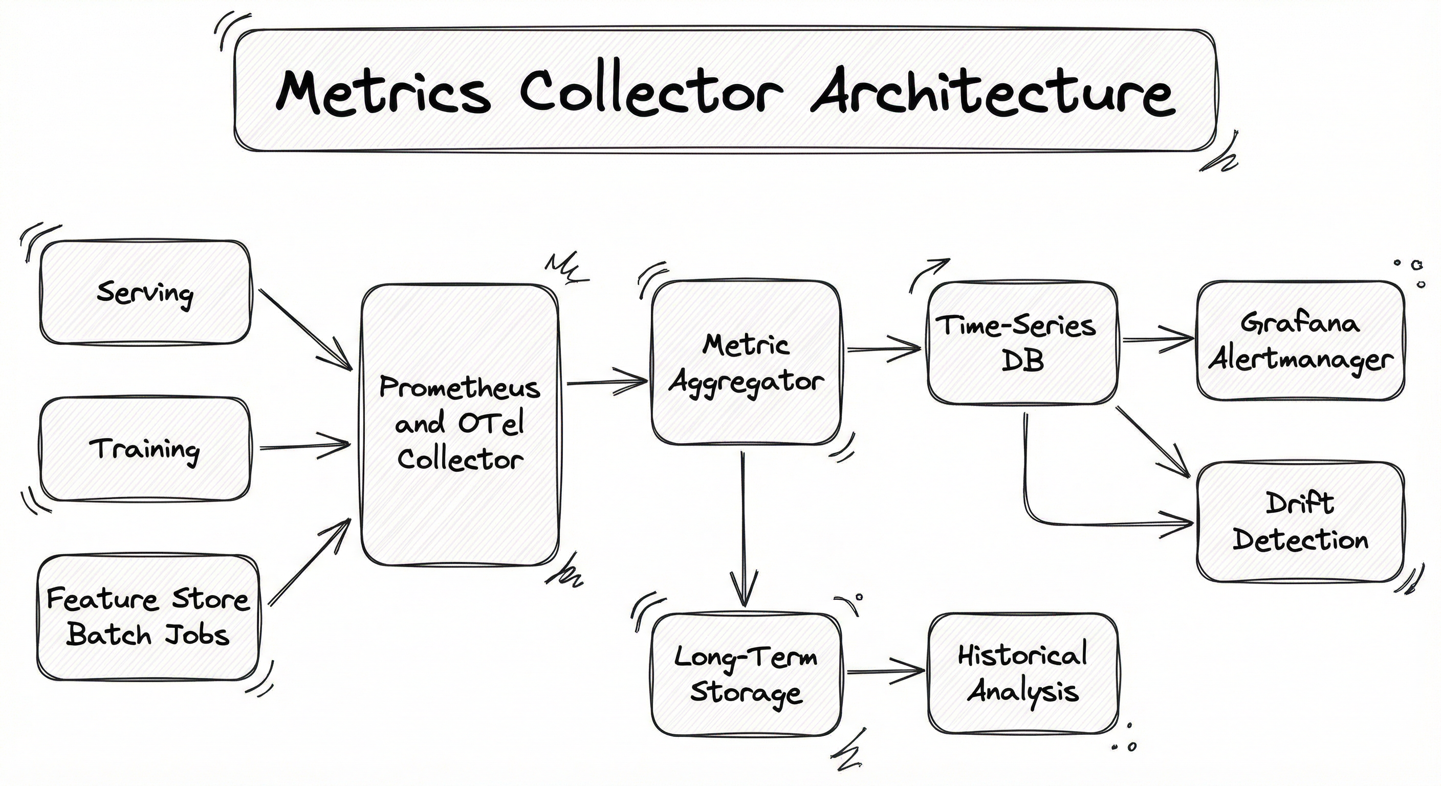
A directed flow diagram showing four source types (Model Serving Endpoint, Training Pipeline, Feature Store, Batch Inference Jobs) feeding into a collection layer (Prometheus Scraper and OTel Collector). The collection layer routes to a Metric Aggregator, which feeds both a Time-Series DB (Prometheus/VictoriaMetrics) and Long-Term Storage (Thanos/S3). The Time-Series DB serves three consumers: Grafana Dashboards, Alertmanager, and Drift Detection. Long-Term Storage serves Historical Analysis.
How to Implement
Choosing Your Implementation Strategy
Implementation approaches fall along a spectrum from DIY to fully managed:
Level 1: Prometheus + Grafana (DIY) -- You instrument your code with prometheus_client, deploy Prometheus to scrape endpoints, and build Grafana dashboards. This is the most common approach for teams that already run Kubernetes. Cost: essentially free for the software, plus infrastructure. A solid m5.xlarge instance on AWS (~INR 7,500/month or ~$90/month) can handle 500K active time-series comfortably.
Level 2: OpenTelemetry + Backend -- You instrument with the OpenTelemetry SDK, deploy the OTel Collector as a gateway, and route to your choice of backend (Prometheus, VictoriaMetrics, Datadog, etc.). This gives you vendor-neutral instrumentation and the flexibility to switch backends without changing application code. The OTel Collector adds maybe 200MB RAM overhead -- negligible for the flexibility it provides.
Level 3: Purpose-built ML monitoring platform -- Tools like Evidently AI, WhyLabs, or Arize AI provide ML-specific metric collection with built-in drift detection, feature monitoring, and model explainability. These are ideal when you want turnkey ML observability without building custom infrastructure. Pricing ranges from free tiers (Evidently Developer, WhyLabs Free) to 399/month (INR 4,200-33,500/month) for production tiers.
Level 4: Cloud-native managed -- Google Vertex AI Model Monitoring, AWS SageMaker Model Monitor, and Azure ML Monitoring provide integrated metric collection within their respective ML platforms. If you're already on one of these clouds, the integration is seamless. But you're locked in, and the per-prediction pricing can surprise you at scale.
For most teams, Level 1 or Level 2 provides the best control-to-effort ratio. You get full ownership of your metric pipeline, the open-source ecosystem is mature, and the operational overhead is manageable with modern tooling.
from prometheus_client import (
    Counter, Histogram, Gauge, Summary,
    start_http_server, CollectorRegistry, REGISTRY
)
import time
import numpy as np

# --- Define Metrics ---

# Counter: total predictions served
PREDICTION_COUNT = Counter(
    'ml_predictions_total',
    'Total number of predictions served',
    ['model_name', 'model_version', 'status']
)

# Histogram: prediction latency in seconds
PREDICTION_LATENCY = Histogram(
    'ml_prediction_latency_seconds',
    'Time spent processing prediction request',
    ['model_name', 'model_version'],
    buckets=[0.005, 0.01, 0.025, 0.05, 0.1, 0.25, 0.5, 1.0, 2.5]
)

# Gauge: current model accuracy (updated periodically)
MODEL_ACCURACY = Gauge(
    'ml_model_accuracy',
    'Current model accuracy score',
    ['model_name', 'model_version', 'metric_type']
)

# Histogram: prediction confidence scores
PREDICTION_CONFIDENCE = Histogram(
    'ml_prediction_confidence',
    'Distribution of prediction confidence scores',
    ['model_name', 'model_version'],
    buckets=[0.1, 0.2, 0.3, 0.4, 0.5, 0.6, 0.7, 0.8, 0.9, 0.95, 0.99]
)

# Counter: feature null rates
FEATURE_NULL_COUNT = Counter(
    'ml_feature_null_total',
    'Count of null/missing values per feature',
    ['model_name', 'feature_name']
)

# Gauge: batch size of incoming requests
BATCH_SIZE = Gauge(
    'ml_request_batch_size',
    'Batch size of current prediction request',
    ['model_name']
)


def predict(model_name: str, model_version: str, features: dict) -> dict:
    """Instrumented prediction function."""
    start_time = time.perf_counter()

    try:
        # Track feature health
        for feat_name, feat_value in features.items():
            if feat_value is None or (isinstance(feat_value, float) and np.isnan(feat_value)):
                FEATURE_NULL_COUNT.labels(
                    model_name=model_name,
                    feature_name=feat_name
                ).inc()

        # --- Run actual model inference ---
        prediction = run_model_inference(features)  # your model call
        confidence = prediction['confidence']

        # Record prediction confidence distribution
        PREDICTION_CONFIDENCE.labels(
            model_name=model_name,
            model_version=model_version
        ).observe(confidence)

        # Increment success counter
        PREDICTION_COUNT.labels(
            model_name=model_name,
            model_version=model_version,
            status='success'
        ).inc()

        return prediction

    except Exception as e:
        PREDICTION_COUNT.labels(
            model_name=model_name,
            model_version=model_version,
            status='error'
        ).inc()
        raise

    finally:
        # Always record latency
        elapsed = time.perf_counter() - start_time
        PREDICTION_LATENCY.labels(
            model_name=model_name,
            model_version=model_version
        ).observe(elapsed)


# Start metrics server on port 8000
start_http_server(8000)
# Your model serving application runs separately
This example demonstrates the four key metric types for ML serving: a counter for prediction counts (segmented by success/error status), a histogram for latency distribution (with ML-appropriate bucket boundaries), a gauge for accuracy scores (updated asynchronously when ground truth labels arrive), and a histogram for confidence score distribution (critical for detecting calibration drift). Notice how the finally block ensures latency is always recorded, even on errors. The label set is deliberately low-cardinality: model name, version, and status -- not user ID or request ID.
from opentelemetry import metrics
from opentelemetry.sdk.metrics import MeterProvider
from opentelemetry.sdk.metrics.export import PeriodicExportingMetricReader
from opentelemetry.exporter.otlp.proto.grpc.metric_exporter import OTLPMetricExporter
from opentelemetry.sdk.resources import Resource
import time

# --- Configure OTel Metrics Pipeline ---
resource = Resource.create({
    "service.name": "fraud-detection-model",
    "service.version": "v2.3.1",
    "deployment.environment": "production",
    "ml.model.framework": "xgboost",
})

exporter = OTLPMetricExporter(
    endpoint="otel-collector.monitoring.svc:4317",
    insecure=True,
)

reader = PeriodicExportingMetricReader(
    exporter,
    export_interval_millis=15000,  # export every 15 seconds
)

provider = MeterProvider(
    resource=resource,
    metric_readers=[reader],
)
metrics.set_meter_provider(provider)

meter = metrics.get_meter("ml.serving", version="1.0.0")

# --- Define ML-Specific Metrics ---
prediction_counter = meter.create_counter(
    name="ml.predictions",
    description="Total predictions served",
    unit="1",
)

latency_histogram = meter.create_histogram(
    name="ml.prediction.duration",
    description="Prediction latency",
    unit="ms",
)

model_score_histogram = meter.create_histogram(
    name="ml.prediction.score",
    description="Distribution of prediction scores",
    unit="1",
)

feature_drift_gauge = meter.create_gauge(
    name="ml.feature.drift_score",
    description="PSI drift score per feature",
    unit="1",
)

batch_throughput = meter.create_counter(
    name="ml.batch.records_processed",
    description="Records processed in batch inference",
    unit="1",
)


def serve_prediction(features: dict) -> dict:
    """ML prediction with OTel instrumentation."""
    start = time.perf_counter()

    result = model.predict(features)

    duration_ms = (time.perf_counter() - start) * 1000

    # Record metrics with attributes
    attributes = {
        "ml.model.name": "fraud_detector",
        "ml.model.version": "v2.3.1",
        "ml.prediction.class": result["label"],
    }

    prediction_counter.add(1, attributes)
    latency_histogram.record(duration_ms, attributes)
    model_score_histogram.record(result["confidence"], attributes)

    return result
This example uses the OpenTelemetry SDK for vendor-neutral instrumentation. The key advantage is that the same instrumentation code works regardless of your backend -- Prometheus, Datadog, New Relic, or any OTLP-compatible receiver. The Resource object attaches static metadata (service name, model framework, deployment environment) to every metric, enabling multi-service correlation. The PeriodicExportingMetricReader pushes metrics every 15 seconds via gRPC to an OTel Collector, which can then route to multiple backends simultaneously.
import pandas as pd
import numpy as np
from prometheus_client import Gauge
from datetime import datetime, timedelta
from typing import Optional
import logging

logger = logging.getLogger(__name__)

# Gauges for delayed-join accuracy metrics
ACCURACY_GAUGE = Gauge(
    'ml_model_accuracy_delayed',
    'Model accuracy computed from delayed ground truth labels',
    ['model_name', 'model_version', 'metric_name', 'window']
)

DRIFT_PSI_GAUGE = Gauge(
    'ml_feature_psi',
    'Population Stability Index for feature drift',
    ['model_name', 'feature_name']
)


def compute_psi(reference: np.ndarray, current: np.ndarray, bins: int = 10) -> float:
    """Compute Population Stability Index between two distributions."""
    breakpoints = np.linspace(
        min(reference.min(), current.min()),
        max(reference.max(), current.max()),
        bins + 1
    )
    ref_counts = np.histogram(reference, bins=breakpoints)[0] / len(reference)
    cur_counts = np.histogram(current, bins=breakpoints)[0] / len(current)

    # Avoid division by zero
    ref_counts = np.clip(ref_counts, 1e-6, None)
    cur_counts = np.clip(cur_counts, 1e-6, None)

    psi = np.sum((cur_counts - ref_counts) * np.log(cur_counts / ref_counts))
    return float(psi)


def compute_delayed_accuracy_metrics(
    predictions_df: pd.DataFrame,
    labels_df: pd.DataFrame,
    model_name: str,
    model_version: str,
    window_hours: int = 24,
) -> dict:
    """
    Join predictions with delayed ground truth labels and compute
    accuracy metrics. This runs as a periodic batch job.

    predictions_df columns: [request_id, prediction, confidence, timestamp]
    labels_df columns: [request_id, ground_truth, label_timestamp]
    """
    # Join predictions with ground truth
    joined = predictions_df.merge(labels_df, on='request_id', how='inner')

    if len(joined) == 0:
        logger.warning(f"No joined labels found for {model_name}/{model_version}")
        return {}

    # Filter to time window
    cutoff = datetime.utcnow() - timedelta(hours=window_hours)
    windowed = joined[joined['timestamp'] >= cutoff]

    if len(windowed) < 100:
        logger.warning(f"Insufficient samples ({len(windowed)}) for reliable metrics")
        return {}

    # Compute classification metrics
    correct = (windowed['prediction'] == windowed['ground_truth']).sum()
    total = len(windowed)
    accuracy = correct / total

    # Precision and recall per class
    from sklearn.metrics import precision_score, recall_score, f1_score, roc_auc_score

    precision = precision_score(windowed['ground_truth'], windowed['prediction'], average='weighted')
    recall = recall_score(windowed['ground_truth'], windowed['prediction'], average='weighted')
    f1 = f1_score(windowed['ground_truth'], windowed['prediction'], average='weighted')

    window_label = f"{window_hours}h"

    # Update Prometheus gauges
    metrics_dict = {
        'accuracy': accuracy,
        'precision': precision,
        'recall': recall,
        'f1_score': f1,
    }

    for metric_name, metric_value in metrics_dict.items():
        ACCURACY_GAUGE.labels(
            model_name=model_name,
            model_version=model_version,
            metric_name=metric_name,
            window=window_label,
        ).set(metric_value)

    logger.info(
        f"Model {model_name}/{model_version} [{window_label}]: "
        f"accuracy={accuracy:.4f}, precision={precision:.4f}, "
        f"recall={recall:.4f}, f1={f1:.4f}, n={total}"
    )

    return metrics_dict


def compute_feature_drift(
    reference_features: pd.DataFrame,
    current_features: pd.DataFrame,
    model_name: str,
    numeric_columns: list[str],
) -> dict:
    """Compute PSI drift scores for numeric features and export to Prometheus."""
    drift_scores = {}

    for col in numeric_columns:
        if col not in reference_features.columns or col not in current_features.columns:
            continue

        ref_values = reference_features[col].dropna().values
        cur_values = current_features[col].dropna().values

        if len(ref_values) < 50 or len(cur_values) < 50:
            continue

        psi = compute_psi(ref_values, cur_values)
        drift_scores[col] = psi

        DRIFT_PSI_GAUGE.labels(
            model_name=model_name,
            feature_name=col,
        ).set(psi)

    return drift_scores
This example addresses the delayed label join problem -- the most common challenge in ML metric collection. Unlike latency or throughput, model accuracy can only be computed when ground truth labels arrive, which may be hours, days, or weeks after the prediction. This batch job joins predictions with delayed labels, computes standard classification metrics (accuracy, precision, recall, F1), and publishes them as Prometheus gauges. It also computes the Population Stability Index (PSI) for feature drift detection, a widely used statistical measure where PSI > 0.2 typically indicates significant distribution shift.
{
  "dashboard": {
    "title": "ML Model Health Dashboard",
    "panels": [
      {
        "title": "Prediction Throughput (req/s)",
        "type": "timeseries",
        "targets": [{
          "expr": "rate(ml_predictions_total{status='success'}[5m])",
          "legendFormat": "{{model_name}} / {{model_version}}"
        }]
      },
      {
        "title": "P99 Prediction Latency",
        "type": "timeseries",
        "targets": [{
          "expr": "histogram_quantile(0.99, rate(ml_prediction_latency_seconds_bucket[5m]))",
          "legendFormat": "p99 - {{model_name}}"
        }],
        "thresholds": [{"value": 0.1, "color": "yellow"}, {"value": 0.5, "color": "red"}]
      },
      {
        "title": "Model Accuracy (Delayed Labels)",
        "type": "gauge",
        "targets": [{
          "expr": "ml_model_accuracy_delayed{metric_name='accuracy', window='24h'}",
          "legendFormat": "{{model_name}} accuracy"
        }],
        "thresholds": [{"value": 0.9, "color": "green"}, {"value": 0.8, "color": "yellow"}, {"value": 0.0, "color": "red"}]
      },
      {
        "title": "Confidence Score Distribution",
        "type": "heatmap",
        "targets": [{
          "expr": "rate(ml_prediction_confidence_bucket[5m])",
          "format": "heatmap"
        }]
      },
      {
        "title": "Feature Drift (PSI)",
        "type": "table",
        "targets": [{
          "expr": "ml_feature_psi > 0.1",
          "legendFormat": "{{feature_name}}"
        }]
      },
      {
        "title": "Error Rate by Model",
        "type": "timeseries",
        "targets": [{
          "expr": "rate(ml_predictions_total{status='error'}[5m]) / rate(ml_predictions_total[5m]) * 100",
          "legendFormat": "{{model_name}} error %"
        }]
      }
    ]
  }
}
This Grafana dashboard JSON demonstrates the six essential panels for ML model health: prediction throughput (are we serving?), P99 latency (are we fast enough?), model accuracy from delayed labels (are we correct?), confidence score heatmap (is the model calibrated?), feature drift table (are inputs healthy?), and error rate (is anything broken?). The PromQL expressions use rate() over 5-minute windows for smooth visualization, and histogram_quantile() for percentile computation from histogram buckets. Threshold annotations provide at-a-glance health indicators.
# prometheus.yml -- Scrape configuration for ML services
global:
  scrape_interval: 15s
  evaluation_interval: 15s

rule_files:
  - '/etc/prometheus/rules/ml_alerts.yml'

scrape_configs:
  - job_name: 'ml-serving'
    kubernetes_sd_configs:
      - role: pod
    relabel_configs:
      - source_labels: [__meta_kubernetes_pod_label_app]
        regex: 'ml-serving-.*'
        action: keep
      - source_labels: [__meta_kubernetes_pod_annotation_prometheus_io_port]
        target_label: __address__
        replacement: '${1}:${2}'
    metrics_path: /metrics
    scrape_interval: 15s

  - job_name: 'ml-training'
    # Push gateway for batch training jobs
    static_configs:
      - targets: ['pushgateway:9091']
    scrape_interval: 30s

  - job_name: 'feature-store'
    static_configs:
      - targets: ['feature-store:8000']
    scrape_interval: 30s

# --- OTel Collector config (otel-collector.yaml) ---
# receivers:
#   otlp:
#     protocols:
#       grpc:
#         endpoint: 0.0.0.0:4317
#       http:
#         endpoint: 0.0.0.0:4318
# processors:
#   batch:
#     timeout: 10s
#     send_batch_size: 1024
#   memory_limiter:
#     check_interval: 5s
#     limit_mib: 512
# exporters:
#   prometheusremotewrite:
#     endpoint: http://victoriametrics:8428/api/v1/write
# service:
#   pipelines:
#     metrics:
#       receivers: [otlp]
#       processors: [memory_limiter, batch]
#       exporters: [prometheusremotewrite]
Common Implementation Mistakes
- ●
High-cardinality label explosion: Adding labels like
user_id,request_id, or individual feature values to Prometheus metrics. Each unique label combination creates a new time-series. With 1M users, a single metric becomes 1M time-series, and Prometheus memory usage balloons from megabytes to tens of gigabytes. Keep labels low-cardinality (model name, version, region, error type). Use logs or traces for high-cardinality data. - ●
Ignoring histogram bucket boundaries: Using default histogram buckets (0.005s to 10s) that don't match your ML workload. A GPU inference endpoint with 2-50ms latencies needs fine-grained buckets in that range. Default buckets will lump 95% of observations into a single bucket, making percentile estimates useless. Always customize buckets for your actual latency distribution.
- ●
Treating accuracy as a real-time metric: Attempting to compute model accuracy in real-time when ground truth labels are delayed by hours or days. This leads to either stale metrics (using old labels) or missing metrics (no labels yet). Design a separate batch pipeline for delayed label joins, and use proxy metrics (confidence distribution, prediction entropy) for real-time quality signals.
- ●
No metric namespacing: Using generic metric names like
latencyorerror_countthat collide across services. Follow a naming convention:{domain}_{component}_{metric_name}_{unit}-- e.g.,ml_serving_prediction_latency_seconds. This prevents confusion and enables consistent querying across your entire fleet. - ●
Scraping too frequently: Setting a 1-second scrape interval when 15-30 seconds is sufficient. Ultra-frequent scraping increases CPU load on both the application (serializing metrics) and Prometheus (ingesting samples), increases storage costs linearly, and rarely provides actionable additional information. For ML workloads, 15-second intervals cover most SLO windows comfortably.
- ●
Not separating operational and ML metrics: Mixing infrastructure metrics (CPU, memory, disk) with ML-specific metrics (accuracy, drift, feature health) in the same dashboard. Different stakeholders need different views. SREs care about uptime and latency; data scientists care about model quality. Separate dashboards with shared context (model version, deployment timestamp) serve both audiences better.
When Should You Use This?
Use When
You have ML models in production and need to track performance beyond basic HTTP health checks -- any model serving real traffic needs metrics collection
Ground truth labels arrive with a delay (hours to weeks) and you need a pipeline to join them with predictions for deferred accuracy computation
Multiple models or model versions are running concurrently and you need a unified view of their relative performance
You need to define and enforce SLOs for ML quality metrics (e.g., 'accuracy must stay above 0.92 over any 7-day window')
Your organization requires audit trails for model behavior -- regulators or compliance teams need historical metric data for model governance
You are building a platform that serves models for multiple teams and need standardized instrumentation across all deployed models
Feature health monitoring is required to detect upstream data pipeline failures before they degrade model predictions
Avoid When
Your model is still in the experimentation phase and has not been deployed to production -- focus on offline evaluation metrics from your experiment tracker (MLflow, W&B) instead
You have a single model with very low traffic (<100 predictions/day) and manual spot-checks are sufficient -- the infrastructure overhead of a full metrics pipeline is not justified yet
You are building a one-off analysis script or notebook that will never run in production -- log to a file and analyze manually
Your organization already has a mature APM solution (Datadog, New Relic) that covers your ML-specific needs through custom metrics -- don't build a parallel system
Budget constraints are extreme and you cannot afford any monitoring infrastructure -- but honestly, even the free tiers of Prometheus + Grafana or Evidently AI cover basic needs, so this bar is very low
Key Tradeoffs
Granularity vs. Cost
The most fundamental tradeoff in metrics collection is granularity vs. storage cost. Collecting per-request metrics at a 1-second resolution gives you beautiful, detailed visibility -- but at 10,000 QPS, that's 864 million data points per day per metric. Even with VictoriaMetrics' excellent compression, you're looking at meaningful storage and query costs.
Most teams find that 15-second aggregated snapshots (Prometheus default) provide sufficient granularity for SLO monitoring. For latency-sensitive debugging, keep a separate high-resolution trace sampling pipeline (e.g., 1% of requests) rather than cranking up the scrape interval for all metrics.
Breadth vs. Depth
| Approach | Breadth | Depth | Cost | Operational Overhead |
|---|---|---|---|---|
| Prometheus + Grafana | High -- any metric you define | Shallow -- no built-in ML semantics | Low (~INR 7,500/$90/month infra) | Medium -- you manage everything |
| OpenTelemetry + Backend | Very high -- vendor-neutral | Medium -- growing ML conventions | Low-Medium | Medium -- collector management |
| Evidently AI / WhyLabs | ML-focused | Deep -- drift, explainability | Medium (INR 4,200-33,500/399/month) | Low -- managed dashboards |
| Cloud-native (Vertex AI, SageMaker) | ML-focused | Deep -- integrated with platform | High -- per-prediction pricing | Very low -- fully managed |
Real-Time vs. Batch Accuracy Metrics
You cannot compute true model accuracy in real-time if labels are delayed. This forces a design choice:
- Real-time proxy metrics: prediction entropy, confidence score distribution, feature null rates. These are available instantly and indicate potential problems, but they don't tell you actual accuracy.
- Batch accuracy metrics: true accuracy, precision, recall, F1 computed via delayed label joins. These are authoritative but stale by definition.
The best systems combine both: real-time proxies for fast alerting, batch accuracy for ground truth validation. When the proxy metrics diverge from batch accuracy trends, it often indicates a calibration problem in the model.
Alternatives & Comparisons
Structured logging captures individual events with rich context (full request/response payloads, feature values, stack traces) but does not provide aggregated time-series views. Use logging for debugging individual predictions; use metrics collection for tracking aggregate trends over time. In practice, you need both -- logs for root cause analysis, metrics for health monitoring.
APM tools (Datadog, New Relic, Dynatrace) provide excellent infrastructure and request-level observability but lack native ML-specific metric types (accuracy, drift, feature health). If your APM tool supports custom metrics, you can layer ML instrumentation on top. Otherwise, a dedicated metrics collector fills the ML-specific gap.
Drift detection is a downstream consumer of metrics, not a replacement for collection. A drift detector consumes feature distribution metrics and prediction distribution metrics produced by the metrics collector, applies statistical tests (PSI, KS, JS divergence), and raises alerts. The metrics collector feeds the drift detector -- they are complementary, not alternatives.
Alerting systems (Prometheus Alertmanager, PagerDuty, OpsGenie) evaluate rules against collected metrics and route notifications. They depend on the metrics collector for data but add the notification and escalation logic that the collector does not provide. Again, complementary -- the collector produces the signal, the alerting system acts on it.
Pros, Cons & Tradeoffs
Advantages
Early detection of silent model degradation -- without metrics, a model can serve bad predictions for weeks before anyone notices. A metrics collector surfaces accuracy drops, drift, and anomalies within minutes to hours, depending on label availability.
Quantified SLOs for ML quality -- transforms vague statements ('the model seems fine') into measurable objectives ('accuracy is 0.94, above our 0.92 SLO target, over the last 7-day window'). This is essential for organizational trust in ML systems.
Historical trend analysis -- with months or years of metric history, you can identify seasonal patterns, gradual degradation trends, and the impact of model retraining or data pipeline changes. This is impossible without persistent metric collection.
Multi-model comparison -- when running A/B tests or deploying new model versions via canary rollout, metrics provide the quantitative basis for promotion or rollback decisions. 'Version B has 2% higher accuracy and 15ms lower P99 latency' is the kind of evidence you need.
Upstream failure propagation detection -- feature null rates and distribution shifts in the metrics collector alert you to data pipeline failures that haven't reached the model yet. This gives you a head start on mitigation before model quality degrades.
Cost optimization signal -- GPU utilization, batch size efficiency, and throughput metrics reveal over-provisioned or under-utilized serving infrastructure. Teams routinely save 20-40% on compute costs by right-sizing based on metric data.
Compliance and audit readiness -- industries like finance (RBI guidelines), healthcare, and insurance require evidence that models are continuously monitored. Historical metrics provide the audit trail.
Disadvantages
Operational overhead -- a full metrics stack (Prometheus, Grafana, Alertmanager, Thanos) requires deployment, monitoring of the monitor, storage management, and upgrade maintenance. This is non-trivial for small teams without dedicated platform engineers.
Storage costs scale with cardinality -- high-cardinality metrics (many models, many features, many label combinations) can make storage costs grow faster than expected. A poorly-designed label schema can cost more than the model serving infrastructure itself.
Delayed accuracy is inherently stale -- the most important ML metric (accuracy) can only be computed after ground truth labels arrive. In some domains (credit risk, long-term recommendations), this delay is weeks or months, making real-time accuracy monitoring impossible.
Alert fatigue risk -- poorly tuned alert thresholds generate excessive notifications, desensitizing the team. The 'boy who cried wolf' effect is very real with ML metrics, where natural variance in accuracy can trigger false alarms.
Metric proxy mismatch -- real-time proxy metrics (confidence scores, prediction entropy) don't always correlate with actual model accuracy. A model can be confidently wrong, leading to a false sense of security from proxy metrics.
Instrumentation maintenance burden -- every new model, feature, or pipeline component needs instrumentation. As the ML system grows, keeping instrumentation comprehensive and consistent across all components becomes a significant maintenance cost.
Failure Modes & Debugging
Cardinality Explosion
Cause
Adding high-cardinality labels (user IDs, session IDs, individual feature names from a 500-feature model) to Prometheus metrics. Each unique label combination creates a separate time-series, and Prometheus stores all active time-series in memory.
Symptoms
Prometheus OOM kills, scrape duration warnings (scrape_duration_seconds spiking), slow PromQL queries, Grafana dashboards timing out. In Kubernetes, the Prometheus pod enters CrashLoopBackOff. On a 16 GB instance, symptoms typically appear around 5-8 million active time-series.
Mitigation
Audit all metric labels and remove any with >1,000 unique values. Use metric_relabel_configs in Prometheus to drop unwanted labels at scrape time. Move high-cardinality data to logs or traces. Consider VictoriaMetrics, which handles high cardinality more gracefully than vanilla Prometheus (10x less RAM for the same number of series).
Scrape Target Disappearance
Cause
Model serving pods are scaled down or restarted (e.g., during a rolling deployment on Kubernetes) and Prometheus loses the scrape target. Metrics go missing for the duration of the gap.
Symptoms
Gaps in time-series data on Grafana dashboards. up metric drops to 0 for affected targets. Alert rules based on absent() may fire. Rate calculations across gaps produce incorrect spikes or drops (the counter resets).
Mitigation
Use Prometheus rate() and increase() functions that handle counter resets gracefully. Deploy a Pushgateway or OpenTelemetry Collector for short-lived jobs. Configure honor_timestamps: true in scrape configs. For Kubernetes, use ServiceMonitor CRDs that automatically discover new pods as they come up.
Metric Staleness and Phantom Values
Cause
A gauge metric (like model accuracy) is set once during initialization and never updated, or a delayed-label batch job fails silently. Prometheus continues serving the last known value for up to 5 minutes (the staleness window), making it look like accuracy is stable when it's actually unknown.
Symptoms
Dashboard shows a flat, unchanging accuracy line. No alerts fire because the value appears normal. The reality is that no new accuracy computation has run for hours or days. Teams develop false confidence in model health.
Mitigation
Accompany every gauge with a last_updated_timestamp gauge that records when the gauge was last genuinely updated. Set alerts on time() - ml_model_accuracy_last_updated > 3600 (no update in 1 hour). Use the absent_over_time() function to detect missing data. Monitor the batch job that produces delayed accuracy metrics as a separate SLO.
Clock Skew Between Collector and Source
Cause
The model serving instance and the Prometheus server have unsynchronized clocks. This causes timestamps to be slightly off, leading to out-of-order samples (which Prometheus rejects) or incorrect rate calculations.
Symptoms
Sporadic 'out of order sample' errors in Prometheus logs. Metrics appear to have negative rates or impossible spikes. Time-series data is inconsistent across panels. This is especially common in multi-region deployments or when running on-premise infrastructure in India without NTP configured.
Mitigation
Ensure NTP (Network Time Protocol) is configured and running on all nodes. Use chrony or systemd-timesyncd. Set honor_timestamps: false in Prometheus scrape configs so Prometheus uses its own clock for sample timestamps. For OpenTelemetry, the collector can normalize timestamps before forwarding.
Metric Pipeline Backpressure
Cause
The OpenTelemetry Collector or Prometheus remote-write pipeline cannot keep up with ingestion volume. This happens during traffic spikes (e.g., Flipkart's Big Billion Days sale) or when the TSDB backend is temporarily unavailable.
Symptoms
Metric data loss -- gaps in time-series that cannot be recovered. OTel Collector logs show sending queue is full warnings. Prometheus remote-write queue depth increases monotonically. Memory usage spikes as buffers fill up.
Mitigation
Configure the OTel Collector's memory_limiter processor with appropriate limits. Use batch processing with a reasonable batch size (1024-4096). Deploy multiple collector replicas behind a load balancer. For Prometheus remote-write, configure queue_config with sufficient capacity and max_samples_per_send. Implement circuit breaker patterns for backend unavailability.
Dashboard Drift from Actual Metrics
Cause
Over time, the metrics emitted by application code evolve (renamed, new labels, changed semantics) but Grafana dashboards are not updated. PromQL queries silently return empty results or incorrect aggregations for renamed metrics.
Symptoms
Dashboard panels show 'No data' or flat zeros. Team members stop trusting dashboards and revert to ad-hoc log analysis. New metrics are collected but never visualized. This is especially common in organizations with separate platform and ML teams.
Mitigation
Version-control your Grafana dashboards alongside application code (use Grafana's provisioning or Grafonnet library). Include dashboard validation in CI/CD pipelines. Implement metric naming conventions as linting rules. Use Grafana's built-in 'no data' alerting to detect broken panels proactively.
Placement in an ML System
Where Does Metrics Collection Sit?
The metrics collector is a cross-cutting concern -- it sits alongside every stage of the ML pipeline, not in a single linear position. It collects signals from:
- Model serving: prediction latency, throughput, error rates, confidence distributions
- Feature engineering: feature null rates, distribution statistics, computation latency
- Training pipelines: training loss, validation metrics, epoch duration, GPU utilization
- Batch inference: records processed, processing time, output distributions
- Data pipelines: data freshness, schema validation, volume metrics
Downstream, the metrics collector feeds into the drift detection system (which runs statistical tests on the collected distributions), the alerting system (which evaluates threshold rules against the metrics), and the dashboarding layer (which visualizes everything for human consumption).
The metrics collector is the foundation layer of the monitoring stack. If it fails or provides incomplete data, everything downstream -- drift detection, alerting, SLO tracking, model governance -- is compromised. This is why the metrics pipeline itself needs to be monitored (yes, you monitor the monitor). A common pattern is to track up{job="ml-serving"} as a meta-metric and alert when scrape targets disappear.
Key Insight: The metrics collector is not a stage in the pipeline -- it is a sidecar to every stage. Its health determines the health of your entire observability stack.
Pipeline Stage
Monitoring / Observability
Upstream
- model-serving
- feature-store
- training-pipeline
- batch-inference
Downstream
- drift-detection
- alerting
- logging
- apm
Scaling Bottlenecks
The primary bottleneck is time-series cardinality. Each unique combination of metric name and label values creates a separate time-series. A system with 50 metrics, 10 model names, 5 versions, and 3 regions generates 50 x 10 x 5 x 3 = 7,500 time-series. That's comfortable. But add per-feature monitoring for a model with 200 features and you're at 1.5 million time-series -- now you need a beefy Prometheus instance or a horizontal solution like VictoriaMetrics.
The second bottleneck is scrape and ingestion throughput. A single Prometheus instance can typically handle 500K-1M active time-series with a 15-second scrape interval. Beyond that, you need federation (multiple Prometheus instances) or a horizontally scalable backend (VictoriaMetrics cluster, Cortex, Mimir).
Some concrete numbers: VictoriaMetrics handles millions of unique time-series with 10x less RAM than InfluxDB and 7x less storage than Prometheus with Thanos. For an Indian startup scaling from 10 to 100 models, VictoriaMetrics on a c5.2xlarge (~INR 14,000/$170/month) can comfortably handle 5-10 million active time-series.
Production Case Studies
Uber's Model Excellence Score (MES) framework quantifies ML model health across the entire lifecycle. Their Michelangelo platform's observability stack (Hue) tracks operational metrics (availability, latency, throughput) and prediction-level indicators (score distributions, calibration, entropy). Feature health checks run in real-time, tracking null rates, detecting drift via statistical tests, and verifying online-offline feature parity. MES adapts SRE principles (SLIs, SLOs, SLAs) specifically for ML quality.
MES enabled Uber to systematically assess and enforce quality across hundreds of production models. The framework reduced mean time to detect model degradation from days to hours, and established organization-wide ML quality standards that scale across thousands of engineers.
Netflix built a dedicated ML Observability platform to bring transparency to their ML models in payments and beyond. Their Atlas time-series telemetry system processes 17 billion metrics and 700 billion distributed traces per day. The ML observability layer includes long-term production performance monitoring, feature and prediction drift monitoring, automated data quality checks, and model explainability tools. Built on top of their open-source Metaflow infrastructure framework.
The ML observability platform enabled Netflix teams to proactively identify model degradation patterns, reducing manual model review overhead and enabling faster iteration on recommendation and personalization models serving 200M+ subscribers.
LinkedIn's Model Health Assurance system monitors ML model inference latency (P50, P75, P90, P99) and feature health in real-time. Their Pro-ML Workspace serves as a one-stop portal tracking training metrics, model evaluation, data quality, and production monitoring. The inference application contains a health assurance component that generates real-time feature distributions and offline data drift metrics, computing statistics on inference-time feature values daily and sending sample quantiles to their monitoring system every minute.
The system automatically detects and alerts on significant drift in model outputs and input feature distributions, enabling AI engineers to efficiently troubleshoot data, model, and code issues before they impact LinkedIn's 900M+ users.
Razorpay built their Mitra data intelligence platform using a Kappa+ architecture with Apache Flink for real-time metric collection and fraud detection. Their ML models process predictions in under 50ms latency, and metric collection is woven into the Flink streaming pipeline itself. Features are computed in real-time streams with Kafka as the data queue and RocksDB for in-memory state management. The metrics pipeline monitors approximately 9,000 fraud detections daily across 10+ billion historical transactions.
Real-time metric collection integrated into the streaming pipeline enables sub-50ms fraud detection latency while maintaining comprehensive model performance monitoring. This approach eliminates the traditional gap between model serving and metric collection that batch-based approaches introduce.
Tooling & Ecosystem
The industry-standard open-source monitoring system and time-series database. Pull-based architecture with powerful PromQL query language. Native support for counters, gauges, histograms, and summaries. The backbone of most Kubernetes monitoring stacks. Integrates with Alertmanager for notification routing. Limited to single-node by default; use Thanos or Cortex for horizontal scaling.
The de facto visualization and dashboarding platform for time-series data. Supports 50+ data sources including Prometheus, InfluxDB, VictoriaMetrics, and Elasticsearch. Provides alerting, annotations, template variables, and a rich plugin ecosystem. Grafana Cloud offers a managed tier. Free tier supports up to 10K metrics with 14-day retention.
CNCF vendor-neutral observability framework providing APIs, SDKs, and the OTel Collector for metrics, traces, and logs. Rapidly adding ML and GenAI semantic conventions (2024-2025). Supports both push and pull models. The Collector can receive data in any format and export to any backend, making it the universal adapter for observability pipelines.
High-performance, cost-effective time-series database compatible with Prometheus. Handles millions of unique time-series with 10x less RAM than InfluxDB and 7x less storage than Prometheus with Thanos. Single-binary deployment or horizontally scalable cluster mode. PromQL and MetricsQL support. Excellent choice for teams outgrowing single-node Prometheus.
Purpose-built ML monitoring platform with native support for data drift detection, model performance tracking, data quality assessments, and target drift. Provides pre-built reports and test suites for tabular, text, and embedding data. Open-source core with a hosted dashboard product. Developer tier is free; Pro starts at $50/month (~INR 4,200/month).
Privacy-first ML monitoring platform based on the open-source whylogs profiling library. Computes statistical profiles of data and model outputs without storing raw data. Enterprise-grade features including SOC 2 Type 2 and HIPAA compliance. Open-sourced under Apache 2.0 in January 2025. Free tier covers 1 project with up to 10M predictions/month.
ML observability platform with specialized support for LLMs, unstructured data (CV, NLP), and SHAP-based explainability. Provides real-time performance monitoring, drift detection, and root cause analysis. Open-source Phoenix edition for local development. Cloud product has a free tier; Pro starts at $50/month (~INR 4,200/month).
Handles alert routing, deduplication, grouping, and silencing for Prometheus-generated alerts. Routes notifications to Slack, PagerDuty, email, OpsGenie, and custom webhooks. Supports inhibition rules (suppress related alerts) and silences (temporary muting during maintenance windows).
Research & References
Faria, Belaid, Bento, Gama (2022)arXiv preprint
Proposes a flexible monitoring framework where a monitor is a collection of metrics computed over the same data. Defines performance monitors (comparing predictions with ground truth), data quality monitors, and operational monitors. Designed to be easily integrated into existing enterprise ML pipelines with minimal disruption.
Shankar, Garcia, Hellerstein, Parameswaran (2021)arXiv preprint
Proposes a new type of data management system offering end-to-end observability for deployed ML pipelines through assisted detection, diagnosis, and reaction to ML-related bugs. Addresses the challenge that ML systems lack real-time feedback (labels) and fail silently.
Various (2025)arXiv preprint
Comprehensive review analyzing 136 papers on ML system monitoring. Categorizes monitoring approaches by motivations, monitored aspects, techniques, metrics, tools, contributions, and current limitations. Provides a taxonomy of runtime issues including data drift, performance degradation, delayed predictions, fairness violations, and safety violations.
Reddi, Cheng, Kanter, Mattson, et al. (2020)MLSys 2020
Defines standardized metrics for ML inference benchmarking: latency, latency-bounded throughput, throughput, and maximum inferences per query, all subject to predefined accuracy targets. Establishes the measurement methodology used by the industry to compare ML serving performance.
Breck, Polyzotis, Roy, Whang (2019)KDD Workshop on Applied Data Science
Introduces the concept of ML health as analogous to physical fitness tracking. Proposes a comprehensive set of health indicators for production ML models covering data validation, training-serving skew, model staleness, and prediction quality. Foundational work from Google on systematic ML monitoring.
Maheshwari, et al. (2023)arXiv preprint
Analyzes the Population Stability Index (PSI) as a metric for detecting data distribution shifts in production ML models. Provides mathematical foundations for PSI computation, threshold selection (PSI > 0.2 indicates significant shift), and practical guidance for integrating PSI into continuous monitoring pipelines.
Shankar, Bui, et al. (2022)arXiv preprint
Interview study with ML practitioners identifying four routine tasks in the ML engineering workflow: data collection, experimentation, evaluation and deployment, and monitoring and response. Highlights that monitoring is often under-resourced and that teams struggle with defining appropriate metrics and alert thresholds.
Interview & Evaluation Perspective
Common Interview Questions
- ●
How would you design a metrics collection system for an ML platform serving 50 models in production?
- ●
What ML-specific metrics would you track beyond standard infrastructure metrics (CPU, memory, latency)?
- ●
How do you handle model accuracy monitoring when ground truth labels are delayed by days or weeks?
- ●
Explain the difference between push-based and pull-based metric collection. When would you use each?
- ●
How would you prevent cardinality explosion in a metrics system tracking hundreds of features across dozens of models?
- ●
What is the difference between monitoring and observability in the context of ML systems?
- ●
How would you define SLOs for an ML model? What SLIs would you track?
Key Points to Mention
- ●
ML metrics fall into four categories: operational (latency, throughput, errors), model quality (accuracy, precision, recall), data quality (null rates, distributions, schema), and business (conversion, revenue, engagement). A complete collector covers all four.
- ●
The delayed label problem is the central challenge -- you cannot compute true accuracy in real-time. Use proxy metrics (confidence distribution, prediction entropy) for immediate signals and batch label-join pipelines for ground truth validation.
- ●
Cardinality management is critical: keep metric labels low-cardinality (model name, version, region), and push high-cardinality data (user IDs, feature values) to logs or traces. This is the #1 operational pitfall teams hit.
- ●
Prometheus with Grafana is the default stack for most teams, but OpenTelemetry is becoming the standard instrumentation layer because it decouples instrumentation from the backend. Always instrument with OTel SDK even if you export to Prometheus.
- ●
The metrics collector must be monitored itself --
upmetric tracking, scrape duration monitoring, and alerting on metric pipeline failures. An unmonitored monitor is a liability.
Pitfalls to Avoid
- ●
Claiming you only need latency and error rate monitoring for ML systems -- this shows you don't understand the ML-specific failure modes (silent degradation, drift, feature staleness) that require domain-specific metrics.
- ●
Proposing to compute real-time accuracy without addressing how ground truth labels are obtained -- labels are almost never available at prediction time, and ignoring this reveals a lack of production experience.
- ●
Suggesting per-request metric storage without discussing cardinality implications -- at 10K QPS, that's 864M data points per day per metric. Always discuss aggregation strategy.
- ●
Treating monitoring as a post-deployment afterthought rather than a design-time concern -- instrumentation should be planned during model development, not bolted on after launch.
Senior-Level Expectation
A senior candidate should discuss the full metrics taxonomy (operational, model quality, data quality, business), the delayed label join pipeline as a first-class architectural component, and the cardinality-cost tradeoff with specific numbers. They should reference SRE principles (SLIs, SLOs, error budgets) adapted for ML -- similar to Uber's MES framework. They should explain how to design metric collection for a multi-model platform with standardized instrumentation (OpenTelemetry semantic conventions), federated storage (Thanos/VictoriaMetrics), and role-based dashboards (SRE vs. data scientist views). They should also discuss the meta-monitoring problem (monitoring the monitor) and cost optimization strategies -- for example, downsampling historical metrics beyond 30 days to reduce storage costs from INR 30,000/month to INR 5,000/month (60) while preserving long-term trend visibility.
Summary
Bringing It All Together
A metrics collector is the instrumentation and aggregation layer that makes ML model health visible and measurable. It captures signals across four dimensions -- operational (latency, throughput, errors), model quality (accuracy, precision, drift), data quality (null rates, distributions, schema), and business (conversion, revenue, engagement) -- and routes them to time-series storage for dashboarding, alerting, and downstream analysis.
The core architectural pattern is straightforward: instrument with Prometheus client or OpenTelemetry SDK, collect via Prometheus scraping or OTel Collector, store in a time-series database (Prometheus, VictoriaMetrics, InfluxDB), visualize with Grafana, and alert with Alertmanager. The complexity lies in the details: managing metric cardinality to control storage costs, handling the delayed label problem for accuracy monitoring, separating real-time proxy metrics from batch ground-truth metrics, and monitoring the monitoring pipeline itself.
The three critical design decisions are: (1) push vs. pull collection -- use pull for long-lived serving endpoints, push for batch jobs and serverless; (2) cardinality budget -- explicitly limit the number of unique time-series per metric to prevent storage explosion; and (3) delayed label pipeline -- build a first-class batch pipeline for joining predictions with ground truth labels, and treat proxy metrics as early warnings rather than substitutes for actual accuracy.
Whether you're running a single fraud detection model at a Bengaluru fintech startup or orchestrating 500 models across a global platform, the metrics collector is the foundation of your ML observability stack. Get it right, and you can detect degradation in minutes rather than weeks. Get it wrong, and you're flying blind -- a terrifying prospect when your models are making real decisions that affect real people.