What is APM and how is it different from simple monitoring?

**Application Performance Monitoring (APM)** goes far beyond basic uptime checks. Simple monitoring answers "is the server running?" APM answers "how is every component of the application performing, and where exactly are the bottlenecks?" The key difference is **depth and correlation**. Simple monitoring gives you individual metrics in isolation (CPU is at 80%, memory is at 60%). APM correlates these into actionable insights: "Request X took 2.3 seconds because it spent 1.8 seconds waiting for the feature store, which was slow because its database connection pool was exhausted." This correlation -- connecting infrastructure metrics to application behavior to user experience -- is what makes APM indispensable for complex ML systems. For ML systems specifically, APM extends to model-level observability: tracking which model version served each request, measuring inference latency broken down by preprocessing vs. forward pass vs. postprocessing, and correlating GPU utilization with prediction throughput.

How much does APM cost for an ML platform?

APM costs vary dramatically based on your approach and scale. Here are realistic numbers for a mid-size ML platform (20-50 hosts, 5,000-10,000 QPS): **Managed vendors**: Datadog APM with infrastructure monitoring runs $31-75/host/month (~INR 2,600-6,300/host/month). For 50 hosts with full-suite features, budget $2,500-3,750/month (~INR 2.1-3.15 lakh/month). New Relic is comparable at $1,250-3,000/month depending on data ingestion volume. **Open-source self-hosted**: The Grafana LGTM stack (Loki + Grafana + Tempo + Mimir) or SigNoz running on cloud infrastructure costs $200-500/month (~INR 16,800-42,000/month) in compute and storage, but requires 10-20 hours/week of engineering time for maintenance. **Indian-specific option**: SigNoz Cloud offers managed hosting with India data residency at significantly lower pricing than Datadog -- starting at a few hundred dollars per month for mid-size workloads. This is particularly attractive for Indian startups navigating data residency requirements under DPDP Act 2023. The hidden cost is **trace storage**. At 10,000 QPS with 10% sampling, expect 75-150 GB/month of trace data. On S3, that's ~$3-5/month for storage, but query costs and retention policies add up.

Why do I need distributed tracing for ML systems specifically?

ML inference pipelines are inherently distributed. A single prediction request typically traverses: 1. **API Gateway** -- authentication, rate limiting, routing 2. **Preprocessing Service** -- input validation, normalization, tokenization 3. **Feature Store** -- real-time feature retrieval (often from Redis or a dedicated feature serving layer) 4. **Model Inference** -- the actual forward pass (potentially on a GPU) 5. **Postprocessing** -- thresholding, formatting, business logic application 6. **Response Assembly** -- combining results, adding metadata Without distributed tracing, when p99 latency spikes from 150ms to 800ms, you have **no way to determine which service caused it**. You'd need to check six separate log files, correlate timestamps manually, and hope the clocks are synchronized. With distributed tracing, you open a single trace and see: "preprocessing took 5ms, feature store took 600ms (cache miss), inference took 120ms, postprocessing took 3ms." The feature store cache miss is immediately obvious. This is especially critical during model deployments. If you ship model v3.2 and latency increases, tracing lets you isolate whether the regression is in the model forward pass itself or in a preprocessing change that accompanied the deployment.

What is tail-based sampling and why does it matter?

**Tail-based sampling** is a trace sampling strategy where the decision to keep or drop a trace is made *after* the entire trace has been collected, based on its characteristics (duration, error status, specific attributes). This contrasts with **head-based sampling**, where the keep/drop decision is made at the first service (the "head") before any downstream spans exist. Why does this matter? With head-based sampling at 10%, you uniformly drop 90% of traces -- including the error traces and slow traces that are diagnostically most valuable. If your error rate is 0.1%, you'll only retain 0.01% of your traffic as error traces. For a 10,000 QPS service, that's just 1 error trace per second instead of 10. Tail-based sampling solves this by applying **policies**: always keep traces with errors, always keep traces slower than a threshold (e.g., 500ms), and probabilistically sample 5-10% of normal traces. The OpenTelemetry Collector's `tail_sampling` processor implements this. The tradeoff: tail-based sampling requires the OTel Collector to buffer complete traces before making sampling decisions, which increases memory usage and adds latency to trace availability. For a service generating 50,000 spans/second with a 10-second decision window, the buffer holds ~500,000 spans -- approximately 1 GB of memory. This is a worthwhile investment for the diagnostic quality improvement.

How do I monitor GPU performance for ML inference?

GPU monitoring for ML workloads requires **NVIDIA DCGM (Data Center GPU Manager)** and its Prometheus exporter, `dcgm-exporter`. Standard APM agents (Datadog Agent, OTel auto-instrumentation) have zero visibility into GPU internals. The critical GPU metrics for ML inference are: - **GPU Utilization** (`DCGM_FI_DEV_GPU_UTIL`): Percentage of time the GPU's streaming multiprocessors are active. Below 30% suggests underutilization (wasted cost). Above 95% suggests a bottleneck. - **GPU Memory Used** (`DCGM_FI_DEV_FB_USED`): Framebuffer memory consumed. When this approaches the GPU's total VRAM, you risk OOM kills that crash inference. - **GPU Temperature** (`DCGM_FI_DEV_GPU_TEMP`): Above 83-85C, most NVIDIA GPUs begin thermal throttling, reducing clock speeds and increasing inference latency by 15-30%. - **SM Clock Frequency** (`DCGM_FI_DEV_SM_CLOCK`): Streaming multiprocessor clock speed. A drop from the boost clock indicates thermal or power throttling. - **PCIe Throughput** (`DCGM_FI_DEV_PCIE_TX_THROUGHPUT`): Host-to-device data transfer rate. A bottleneck here means the GPU is starved for input data. Deploy `dcgm-exporter` as a Kubernetes DaemonSet on GPU nodes (see the implementation section for the full manifest). Scrape metrics with Prometheus or the OTel Collector, and visualize in Grafana alongside your application metrics. The correlation between GPU temperature spikes and inference latency increases is often the "aha moment" that justifies GPU monitoring investment.

What are the golden signals for ML service monitoring?

The **four golden signals** (from the Google SRE book) adapted for ML services are: 1. **Latency**: p50, p95, and p99 of end-to-end inference time. For ML, also break this down by phase: preprocessing latency, feature retrieval latency, model forward pass latency, and postprocessing latency. Track latency per model version to detect regressions. 2. **Traffic**: Requests per second (QPS) to the inference endpoint. For ML, also track batch sizes and token throughput (for LLM services). Sudden traffic drops can indicate upstream failures, while spikes require autoscaling response. 3. **Errors**: Error rate (5xx responses / total responses). For ML, also track **soft errors**: requests that return 200 but with fallback predictions, missing features, or stale cache hits. A model returning a default prediction for 15% of requests because the feature store timed out is a critical issue that HTTP status codes won't catch. 4. **Saturation**: How close key resources are to capacity. For ML: GPU utilization and memory, CPU and RAM on preprocessing nodes, feature store connection pool usage, inference queue depth. When saturation exceeds 80%, start scaling or risk degradation. Many teams add a fifth signal specific to ML: **Prediction Distribution**. If your fraud detection model suddenly flags 40% of transactions as fraudulent (up from the usual 2%), something is very wrong -- even if latency, errors, and throughput look normal. This is the signal that bridges APM and ML model monitoring.

How do I avoid alert fatigue from APM?

Alert fatigue is the #1 operational risk of APM adoption. Here's a battle-tested framework: **1. Use SLO-based alerting, not raw thresholds.** Instead of alerting when p99 > 200ms (which might fire during every minor GC pause), alert when the **error budget burn rate** exceeds 14.4x the allowed rate for a 1-hour window or 6x for a 6-hour window. This multi-window approach (from Google's SRE workbook) fires only when sustained degradation threatens your monthly SLO. **2. Classify alerts by severity.** Critical alerts (page the on-call) should be reserved for customer-impacting SLO breaches. Warning alerts (create a ticket) for approaching thresholds. Informational alerts (Slack channel) for anomalies that need investigation but not immediate action. A good ratio is: fewer than 2 critical pages per on-call shift. **3. Every alert must have a runbook.** If an engineer can't take a concrete action when an alert fires, the alert should not exist. The runbook should specify: what to check first, common root causes, mitigation steps, and escalation paths. **4. Review alerts quarterly.** Any alert that fires more than 3 times per week without leading to remedial action should be tuned (raise threshold, increase evaluation window) or deleted. Dead alerts erode trust in the entire alerting system. **5. Use anomaly detection for dynamic baselines.** ML inference traffic often follows daily and weekly patterns (e.g., a Swiggy recommendation model sees 10x traffic at lunch and dinner). Static thresholds will fire false alerts during natural traffic fluctuations. Tools like Datadog's Watchdog or custom Prophet-based baselines adapt to seasonality.

What is OpenTelemetry and why should I use it for ML systems?

**OpenTelemetry (OTel)** is a CNCF project that provides a vendor-neutral standard for generating, collecting, and exporting telemetry data (traces, metrics, and logs). It was formed in 2019 by merging two competing projects: OpenTracing and OpenCensus. For ML systems, OTel is the right choice for three reasons: **1. Vendor independence.** You instrument your ML inference service with the OTel SDK once. If you start with SigNoz and later move to Datadog (or vice versa), you change the exporter configuration -- not a single line of application code. Given how fast the observability landscape is evolving, this flexibility is valuable. **2. Semantic conventions for ML.** OTel is actively developing semantic conventions for GenAI and ML workloads (OTel 1.37+ includes conventions for LLM token usage, model identifiers, and embedding dimensions). This means your ML-specific span attributes follow a standard schema that any OTel-compatible backend understands. **3. Ecosystem breadth.** OTel provides auto-instrumentation for popular ML serving frameworks: FastAPI, Flask, gRPC (common for TFServing/Triton), and HTTP clients (for feature store calls). The OTel Collector integrates with Prometheus scrapers (for DCGM metrics) and supports tail-based sampling processors. It's the single telemetry pipeline that unifies your entire ML platform's observability. The OTel Collector also supports data residency routing -- you can configure it to send traces from Indian users to an India-region backend while routing other data elsewhere. This is increasingly important under India's DPDP Act.

Monitoring

APM in Machine Learning

Application Performance Monitoring (APM) is the discipline of instrumenting, measuring, and analyzing the runtime behavior of software services -- and in the ML world, that includes everything from feature stores to inference endpoints to GPU utilization during batch training.

Why does APM matter specifically for ML systems? Because ML services fail in ways traditional web applications don't. A recommendation endpoint might return HTTP 200 with perfect latency while serving stale embeddings from a corrupted cache. A fraud detection model might silently degrade from 98% precision to 72% because an upstream feature pipeline started producing nulls. APM is your first line of defense against these invisible failures.

Modern APM goes far beyond simple uptime checks. It encompasses distributed tracing (following a single request through dozens of microservices), latency profiling (understanding p50, p95, and p99 response times), resource monitoring (CPU, memory, GPU utilization, network I/O), and dependency mapping (which services call which). For ML systems, you add layers like inference latency breakdowns (preprocessing vs. model forward pass vs. postprocessing), GPU memory profiling, batch queue depths, and model version tracking.

From Razorpay tracing payment fraud detection pipelines across hundreds of microservices to Uber using Jaeger to trace ride-matching ML models across global data centers -- APM is the connective tissue that makes complex ML systems operable. Without it, you're flying blind in production.

Concept Snapshot

What It Is: A monitoring discipline that instruments, collects, and analyzes performance telemetry (traces, metrics, and profiling data) from application services to diagnose latency, errors, and resource bottlenecks in real time.
Category: Monitoring
Complexity: Intermediate
Inputs / Outputs: Inputs: instrumented application code emitting spans, metrics, and logs. Outputs: service maps, latency distributions (p50/p95/p99), error rate dashboards, flame graphs, and automated alerts.
System Placement: Sits as an observability layer alongside (not inline with) the ML serving pipeline, collecting telemetry from model-serving, feature-store, and preprocessing services.
Also Known As: application performance management, distributed tracing, service observability, request tracing, performance profiling
Typical Users: ML Engineers, SRE / Platform Engineers, DevOps Engineers, Backend Engineers, Infrastructure Engineers
Prerequisites: HTTP and gRPC fundamentals, Microservices architecture basics, Basic statistics (percentiles, distributions), Container orchestration (Kubernetes)
Key Terms: spantracetrace context propagationOpenTelemetryp50/p95/p99 latencyflame graphservice mapSLI/SLO/SLADCGMtail latency

Why This Concept Exists

The Observability Crisis in ML Systems

Traditional web applications have a relatively straightforward failure model: either the server responds or it doesn't. You check HTTP status codes, measure response times, and you're mostly covered. ML systems shatter this simplicity.

Consider a typical ML inference pipeline: a request hits an API gateway, gets routed to a preprocessing service that fetches features from a feature store, passes through an embedding model, hits a vector store for retrieval, feeds results to a re-ranker, and finally returns a response. That's six services minimum. When p99 latency spikes from 200ms to 2 seconds, where is the bottleneck? Without distributed tracing, you're reduced to guessing.

The Evolution from Logs to Observability

The journey started with logs -- plain text files dumped to disk. Teams would SSH into servers and grep through log files when something went wrong. This worked for monoliths but collapsed spectacularly when organizations moved to microservices.

Google's Dapper paper (Sigelman et al., 2010) introduced the foundational concept of distributed tracing -- assigning a unique trace ID to each request and propagating it across service boundaries. This single idea transformed observability. Twitter open-sourced Zipkin in 2012 based on Dapper's principles. Uber built and open-sourced Jaeger in 2016. By 2019, the OpenTelemetry project merged OpenTracing and OpenCensus into a vendor-neutral standard that now dominates the industry.

Why ML Systems Need Specialized APM

Standard APM tools were built for request-response web services. ML systems introduce unique challenges:

GPU resource monitoring: Traditional APM doesn't understand GPU utilization, VRAM allocation, or CUDA kernel execution times. You need specialized exporters like NVIDIA DCGM.
Model version correlation: When latency changes, was it the new model deployment or an infrastructure issue? APM must track model versions as first-class metadata.
Batch vs. real-time asymmetry: Training jobs run for hours on GPUs. Inference requests complete in milliseconds. The same APM system must handle both time scales.
Silent quality degradation: A model returning wrong predictions at low latency looks perfectly healthy to standard APM. You need ML-specific signals (prediction distributions, feature drift scores) alongside infrastructure metrics.

Key Insight: APM for ML systems is not just "regular APM plus a GPU dashboard." It requires fundamentally rethinking what "healthy" means -- a fast, available service that returns garbage predictions is worse than a slow service that returns correct ones.

Core Intuition & Mental Model

The Three Pillars Mental Model

Think of APM as providing three complementary lenses into your system:

Metrics tell you what is happening: request rate is 5,000 QPS, p99 latency is 180ms, GPU utilization is 73%. Metrics are cheap, aggregated, and great for dashboards and alerts.
Traces tell you where it's happening: this specific request spent 12ms in preprocessing, 45ms waiting for the feature store, 80ms in model inference, and 15ms in postprocessing. Traces are per-request and expensive at scale.
Profiles tell you why it's happening: 60% of inference time is spent in the attention layer, memory allocation is the bottleneck in the preprocessing service. Profiles are deep but heavyweight.

No single pillar is sufficient. Metrics without traces give you averages that hide outliers. Traces without metrics give you anecdotes without trends. Profiles without traces give you local optimization without understanding the system.

The Restaurant Analogy

Imagine you run a large restaurant (your ML system). Metrics are like knowing your average wait time is 15 minutes and you served 200 customers today. Traces are like following a single customer's journey: they waited 5 minutes for a table, 10 minutes for their order to be taken, the kitchen took 20 minutes, and food was served in 2 minutes. Profiles are like watching the kitchen chef and seeing that 70% of their time is spent chopping vegetables because the knives are dull.

A Swiggy delivery partner experiencing a slow order routing can be traced through the recommendation model, the restaurant matching service, and the delivery optimization engine -- each span in the trace revealing exactly where time was spent.

Expert Note: In practice, you'll use metrics for alerting ("something is wrong"), traces for diagnosis ("here's where it's wrong"), and profiles for optimization ("here's why it's slow"). Build your APM strategy around this workflow, not around a single tool.

Technical Foundations

Formalizing Latency Measurement

APM systems fundamentally measure latency distributions. Let $L$ be the random variable representing request latency. The percentile function $P_q$ gives the value below which $q\%$ of observations fall:

$P_q(L) = \inf \{ x : F_L(x) \geq q/100 \}$

where $F_L(x) = \Pr(L \leq x)$ is the cumulative distribution function.

In practice, we care about three percentiles:

p50 (median): The "typical" request. Half are faster, half are slower.
p95: The experience of your worst 5% of users.
p99: The experience of your worst 1% of users -- the tail latency that drives SLA violations.

Why Tail Latency Matters Disproportionately

For a system making $n$ sequential service calls, the probability that at least one call hits the p99 tail is:

$\Pr(\text{at least one tail}) = 1 - (1 - 0.01)^n = 1 - 0.99^n$

For $n = 10$ services (common in ML pipelines): $1 - 0.99^{10} \approx 0.0956$ -- roughly 10% of end-to-end requests will experience at least one tail-latency hop. For $n = 50$ : $1 - 0.99^{50} \approx 0.395$ -- nearly 40% of requests. This is why Jeff Dean famously said "the tail at scale" is the dominant challenge.

Apdex Score

The Application Performance Index (Apdex) provides a normalized satisfaction score:

$\text{Apdex} = \frac{S + \frac{T}{2}}{N}$

where $S$ = satisfied requests (latency $\leq$ threshold $t$ ), $T$ = tolerating requests ( $t <$ latency $\leq 4t$ ), and $N$ = total requests. An Apdex of 0.94+ is considered "excellent," while below 0.50 is "unacceptable."

SLI, SLO, and SLA

APM enables the formal definition of service reliability:

Service Level Indicator (SLI): A quantitative measure, e.g., "proportion of requests completed in under 200ms."
Service Level Objective (SLO): A target for the SLI, e.g., "99.9% of requests under 200ms over a 30-day window."
Service Level Agreement (SLA): A contractual commitment with consequences, e.g., "if uptime drops below 99.95%, customer receives credits."

The error budget is:

$\text{Error Budget} = 1 - \text{SLO target}$

For a 99.9% SLO over 30 days: $0.001 \times 30 \times 24 \times 60 = 43.2$ minutes of allowed downtime per month.

Internal Architecture

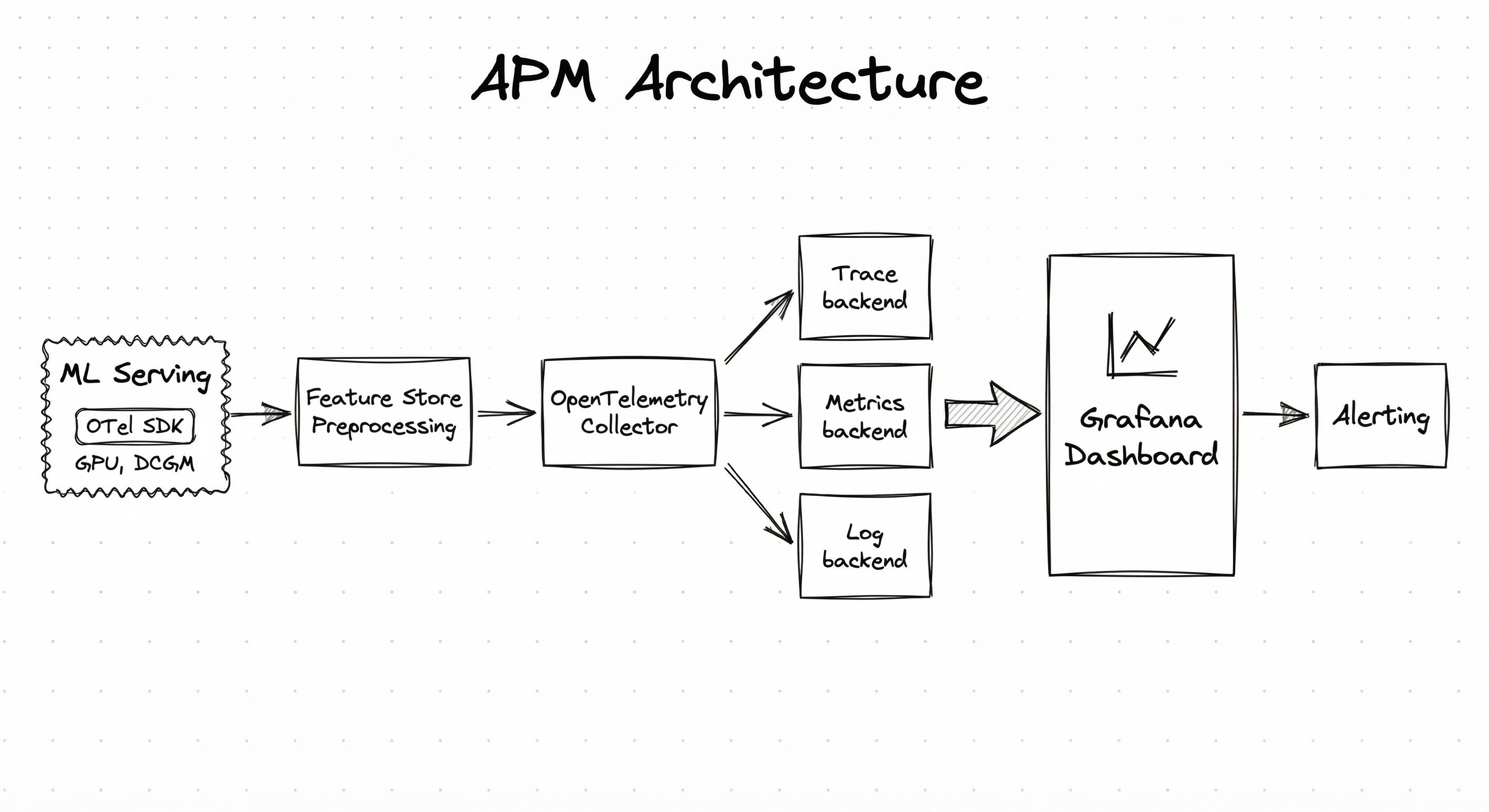
A production APM system for ML services consists of four layers: an instrumentation layer embedded in application code, a collection layer that aggregates and ships telemetry, a storage and processing layer that indexes traces and computes metrics, and a visualization and alerting layer that surfaces insights to engineers.

The architecture follows a push model: instrumented services emit telemetry to a collector (typically the OpenTelemetry Collector), which batches, processes, and exports data to one or more backends. This decouples instrumentation from storage, allowing you to switch backends (e.g., from Jaeger to Grafana Tempo) without changing application code.

APM for ML Systems Architecture — A layered architecture showing ML services (serving, feature store, preprocessing) instrumented w...

For ML-specific monitoring, the architecture extends with NVIDIA DCGM Exporter for GPU telemetry, custom span attributes for model version and batch size metadata, and continuous profiling agents (like Pyroscope or Datadog Continuous Profiler) that capture flame graphs without manual instrumentation.

Key Components

Instrumentation Layer (OTel SDK)

Embeds in application code to create spans (units of work with start time, duration, and metadata), record metrics (counters, histograms, gauges), and attach context (trace ID, span ID, baggage) that propagates across service boundaries via HTTP headers or gRPC metadata.

OpenTelemetry Collector

A vendor-neutral telemetry pipeline that receives data from instrumented services via OTLP (OpenTelemetry Protocol), applies processors (batching, sampling, attribute enrichment), and exports to one or more backends. Runs as a sidecar or daemonset in Kubernetes.

Trace Backend (Jaeger / Grafana Tempo)

Stores and indexes distributed traces. Provides query APIs for searching traces by service name, operation, duration, tags, and trace ID. Supports trace comparison and critical path analysis.

Metrics Backend (Prometheus / Mimir)

Collects and stores time-series metrics using a pull (Prometheus) or push (OTLP) model. Supports PromQL for querying, alerting rules, and recording rules for pre-aggregation. Grafana Mimir provides long-term storage and horizontal scaling.

GPU Telemetry Exporter (NVIDIA DCGM)

NVIDIA Data Center GPU Manager exports GPU metrics (utilization, memory usage, temperature, power draw, ECC errors, SM clock frequency) in Prometheus format. Essential for monitoring ML inference and training workloads on GPU nodes.

Continuous Profiler

Captures stack-level profiling data (CPU, memory, wall-clock time) continuously with low overhead (~2-5%). Enables engineers to correlate hot code paths with specific traces and identify the why behind latency spikes.

Visualization and Alerting Layer

Grafana dashboards, Datadog APM views, or New Relic interfaces that render service maps, latency heatmaps, error rate charts, and GPU utilization graphs. Alerting integrations with PagerDuty, OpsGenie, and Slack notify on-call engineers when SLOs are breached.

Data Flow

Trace Propagation Path: When a request enters the ML serving gateway, the OTel SDK generates a trace ID and root span. As the request moves to the preprocessing service, the trace context is propagated via W3C Traceparent headers. Each downstream service (feature store, model inference, postprocessing) creates child spans under the same trace ID. GPU execution time is captured as a span attribute on the inference span.

Metrics Path: Each service emits metrics (request count, latency histogram, error count) to the OTel Collector, which batches and exports them to Prometheus or a remote-write compatible backend every 15-60 seconds. DCGM Exporter runs as a daemonset on GPU nodes and exposes GPU metrics on port 9400, which the OTel Collector scrapes.

Alert Path: Alerting rules in Prometheus or the APM backend evaluate conditions (e.g., p99_latency > 500ms for 5 minutes) and fire alerts to PagerDuty or Slack via webhooks. Critical alerts page the on-call engineer; warnings create tickets.

A layered architecture showing ML services (serving, feature store, preprocessing) instrumented with OTel SDKs, plus a GPU node with DCGM Exporter, all feeding into a central OpenTelemetry Collector. The collector fans out to three backends: a trace store (Jaeger/Tempo), a metrics store (Prometheus/Mimir), and a log store (Loki/Elasticsearch). All three backends feed into a unified dashboard (Grafana/Datadog) which connects to an alerting system (PagerDuty/Slack).

How to Implement

Two Implementation Philosophies

You can approach APM for ML systems in two ways:

Philosophy A: Vendor-managed APM (Datadog, New Relic, Dynatrace) -- you install an agent, configure auto-instrumentation, and get dashboards, traces, and alerts out of the box. This is the fastest path to value but comes with significant cost at scale. Datadog APM pricing starts at ~ $31/host/month (~INR 2,600/host/month) for basic APM and can reach$ 40-75/host/month (~INR 3,350-6,300/host/month) with full-suite features. For a team running 50 hosts, that's $1,550-3,750/month (~INR 1.3-3.15 lakh/month).

Philosophy B: Open-source stack (OpenTelemetry + Prometheus + Grafana Tempo + Grafana) -- you own the entire stack. Initial setup is more involved (2-4 weeks for a small team), but ongoing costs are limited to infrastructure. An Indian startup like SigNoz (YC W21, based in Bengaluru) offers an open-source, OpenTelemetry-native alternative to Datadog that can be self-hosted or used as a managed service with data residency in India.

For ML-specific monitoring, both approaches require additional instrumentation: custom span attributes for model version, batch size, and feature counts; NVIDIA DCGM integration for GPU metrics; and application-level metrics for prediction distributions and feature statistics.

Cost Note for Indian Teams: Datadog's Enterprise plan for a 20-host ML platform costs approximately $15,000-18,000/year (~INR 12.6-15.1 lakh/year). A self-hosted SigNoz or Grafana LGTM stack on equivalent infrastructure runs ~$ 3,000-5,000/year (~INR 2.5-4.2 lakh/year) in cloud costs, but requires 0.5-1 FTE of operational investment.

OpenTelemetry — Instrument an ML Inference Service with Custom Spans61 lines

from opentelemetry import trace
from opentelemetry.sdk.trace import TracerProvider
from opentelemetry.sdk.trace.export import BatchSpanProcessor
from opentelemetry.exporter.otlp.proto.grpc.trace_exporter import OTLPSpanExporter
from opentelemetry.sdk.resources import Resource
from opentelemetry.semconv.resource import ResourceAttributes
import time
import numpy as np

# Configure the tracer
resource = Resource.create({
    ResourceAttributes.SERVICE_NAME: "ml-inference-service",
    ResourceAttributes.SERVICE_VERSION: "1.4.2",
    "ml.model.name": "fraud-detector-v3",
    "ml.model.version": "3.1.0",
    "deployment.environment": "production",
})

provider = TracerProvider(resource=resource)
exporter = OTLPSpanExporter(endpoint="http://otel-collector:4317", insecure=True)
provider.add_span_processor(BatchSpanProcessor(exporter))
trace.set_tracer_provider(provider)
tracer = trace.get_tracer("ml.inference")


def predict(request_data: dict) -> dict:
    """Run inference with full APM instrumentation."""
    with tracer.start_as_current_span("inference.predict") as root_span:
        root_span.set_attribute("ml.request.batch_size", len(request_data["inputs"]))
        root_span.set_attribute("ml.model.name", "fraud-detector-v3")

        # Phase 1: Feature preprocessing
        with tracer.start_as_current_span("inference.preprocess") as preprocess_span:
            start = time.perf_counter()
            features = preprocess(request_data["inputs"])
            duration_ms = (time.perf_counter() - start) * 1000
            preprocess_span.set_attribute("ml.preprocess.duration_ms", duration_ms)
            preprocess_span.set_attribute("ml.preprocess.feature_count", features.shape[1])
            preprocess_span.set_attribute("ml.preprocess.null_count", int(np.isnan(features).sum()))

        # Phase 2: Model forward pass
        with tracer.start_as_current_span("inference.forward_pass") as model_span:
            start = time.perf_counter()
            predictions = model.predict(features)
            duration_ms = (time.perf_counter() - start) * 1000
            model_span.set_attribute("ml.inference.duration_ms", duration_ms)
            model_span.set_attribute("ml.inference.gpu_used", True)
            model_span.set_attribute("ml.inference.model_version", "3.1.0")

        # Phase 3: Postprocessing and thresholding
        with tracer.start_as_current_span("inference.postprocess") as post_span:
            start = time.perf_counter()
            results = postprocess(predictions, threshold=0.85)
            duration_ms = (time.perf_counter() - start) * 1000
            post_span.set_attribute("ml.postprocess.duration_ms", duration_ms)
            post_span.set_attribute("ml.postprocess.flagged_count", sum(results["flags"]))

        root_span.set_attribute("ml.predict.total_duration_ms",
            root_span.end_time - root_span.start_time if hasattr(root_span, 'end_time') else 0)

        return results

This example instruments an ML inference function with OpenTelemetry, creating a parent span for the entire prediction and child spans for each phase (preprocessing, forward pass, postprocessing). Custom attributes like ml.model.version, ml.preprocess.null_count, and ml.postprocess.flagged_count provide ML-specific observability that standard APM auto-instrumentation misses. The trace context propagates automatically to downstream services (feature store, etc.) via W3C Traceparent headers.

Prometheus — Custom Metrics for ML Inference Latency Histograms65 lines

from prometheus_client import Histogram, Counter, Gauge, start_http_server
import time

# Define ML-specific metrics
INFERENCE_LATENCY = Histogram(
    "ml_inference_latency_seconds",
    "Latency of model inference in seconds",
    labelnames=["model_name", "model_version", "endpoint"],
    buckets=[0.01, 0.025, 0.05, 0.1, 0.25, 0.5, 1.0, 2.5, 5.0, 10.0],
)

PREPROCESS_LATENCY = Histogram(
    "ml_preprocess_latency_seconds",
    "Latency of feature preprocessing in seconds",
    labelnames=["model_name"],
    buckets=[0.005, 0.01, 0.025, 0.05, 0.1, 0.25, 0.5],
)

PREDICTION_COUNT = Counter(
    "ml_predictions_total",
    "Total number of predictions served",
    labelnames=["model_name", "model_version", "result_class"],
)

MODEL_LOAD_TIME = Gauge(
    "ml_model_load_duration_seconds",
    "Time taken to load the model into memory",
    labelnames=["model_name", "model_version"],
)

GPU_MEMORY_USED = Gauge(
    "ml_gpu_memory_used_bytes",
    "GPU memory used by the model",
    labelnames=["gpu_id", "model_name"],
)

# Start metrics server on port 8000
start_http_server(8000)


def serve_prediction(request):
    model_name = "fraud-detector"
    model_version = "v3.1"

    # Time preprocessing
    with PREPROCESS_LATENCY.labels(model_name=model_name).time():
        features = preprocess(request)

    # Time inference
    with INFERENCE_LATENCY.labels(
        model_name=model_name,
        model_version=model_version,
        endpoint="/predict",
    ).time():
        prediction = model.predict(features)

    # Record prediction class
    result_class = "fraud" if prediction > 0.85 else "legitimate"
    PREDICTION_COUNT.labels(
        model_name=model_name,
        model_version=model_version,
        result_class=result_class,
    ).inc()

    return {"prediction": float(prediction), "class": result_class}

This example sets up Prometheus histograms for inference and preprocessing latency with ML-appropriate bucket boundaries (10ms to 10s for inference, 5ms to 500ms for preprocessing). Counters track predictions by class, enabling you to monitor prediction distribution drift. Gauges track model load time and GPU memory -- critical for capacity planning. The histogram buckets are chosen to give meaningful percentile resolution around typical ML inference latencies.

NVIDIA DCGM Exporter — Kubernetes DaemonSet for GPU Monitoring58 lines

apiVersion: apps/v1
kind: DaemonSet
metadata:
  name: dcgm-exporter
  namespace: monitoring
  labels:
    app: dcgm-exporter
spec:
  selector:
    matchLabels:
      app: dcgm-exporter
  template:
    metadata:
      labels:
        app: dcgm-exporter
      annotations:
        prometheus.io/scrape: "true"
        prometheus.io/port: "9400"
    spec:
      nodeSelector:
        nvidia.com/gpu.present: "true"
      containers:
      - name: dcgm-exporter
        image: nvcr.io/nvidia/k8s/dcgm-exporter:3.3.8-3.6.0-ubuntu22.04
        ports:
        - containerPort: 9400
          name: metrics
        securityContext:
          capabilities:
            add: ["SYS_ADMIN"]
        env:
        - name: DCGM_EXPORTER_COLLECTORS
          value: "/etc/dcgm-exporter/dcp-metrics-included.csv"
        volumeMounts:
        - name: dcgm-config
          mountPath: /etc/dcgm-exporter
      volumes:
      - name: dcgm-config
        configMap:
          name: dcgm-metrics-config
---
apiVersion: v1
kind: ConfigMap
metadata:
  name: dcgm-metrics-config
  namespace: monitoring
data:
  dcp-metrics-included.csv: |
    DCGM_FI_DEV_GPU_UTIL, gauge, GPU utilization (%)
    DCGM_FI_DEV_MEM_COPY_UTIL, gauge, Memory utilization (%)
    DCGM_FI_DEV_FB_USED, gauge, Framebuffer memory used (MiB)
    DCGM_FI_DEV_FB_FREE, gauge, Framebuffer memory free (MiB)
    DCGM_FI_DEV_GPU_TEMP, gauge, GPU temperature (C)
    DCGM_FI_DEV_POWER_USAGE, gauge, Power usage (W)
    DCGM_FI_DEV_SM_CLOCK, gauge, SM clock frequency (MHz)
    DCGM_FI_DEV_MEM_CLOCK, gauge, Memory clock frequency (MHz)
    DCGM_FI_DEV_PCIE_TX_THROUGHPUT, counter, PCIe TX throughput (KB/s)
    DCGM_FI_DEV_PCIE_RX_THROUGHPUT, counter, PCIe RX throughput (KB/s)

This Kubernetes DaemonSet deploys NVIDIA DCGM Exporter on every GPU node in your cluster. It exposes GPU metrics (utilization, memory, temperature, power, PCIe throughput) in Prometheus format on port 9400. The nodeSelector ensures it only runs on nodes with GPUs. The ConfigMap customizes which DCGM metrics to export -- you should include at minimum GPU utilization, memory usage, and temperature for ML workloads. Prometheus or the OTel Collector then scrapes these metrics alongside your application metrics.

Grafana Alerting — SLO-Based Alert Rules for ML Inference84 lines

# Prometheus alerting rules for ML inference SLOs
groups:
- name: ml_inference_slos
  interval: 30s
  rules:
  # P99 latency SLO: inference must complete within 500ms
  - alert: InferenceP99LatencyHigh
    expr: |
      histogram_quantile(0.99,
        sum(rate(ml_inference_latency_seconds_bucket{
          model_name="fraud-detector"
        }[5m])) by (le, model_version)
      ) > 0.5
    for: 5m
    labels:
      severity: critical
      team: ml-platform
    annotations:
      summary: "P99 inference latency exceeds 500ms SLO"
      description: |
        Model {{ $labels.model_version }} p99 latency is
        {{ $value | humanizeDuration }}. SLO threshold: 500ms.
        Check GPU utilization and model batch size.
      runbook_url: "https://wiki.internal/runbooks/ml-latency-slo"

  # Error rate SLO: less than 0.1% of predictions should fail
  - alert: InferenceErrorRateHigh
    expr: |
      sum(rate(ml_predictions_total{result_class="error"}[5m]))
      /
      sum(rate(ml_predictions_total[5m]))
      > 0.001
    for: 3m
    labels:
      severity: warning
      team: ml-platform
    annotations:
      summary: "Inference error rate exceeds 0.1% SLO"
      description: |
        Current error rate: {{ $value | humanizePercentage }}.
        Check preprocessing pipeline and model health.

  # GPU memory pressure: alert before OOM
  - alert: GPUMemoryPressure
    expr: |
      (DCGM_FI_DEV_FB_USED / (DCGM_FI_DEV_FB_USED + DCGM_FI_DEV_FB_FREE))
      > 0.90
    for: 2m
    labels:
      severity: warning
      team: infrastructure
    annotations:
      summary: "GPU memory usage exceeds 90%"
      description: |
        GPU {{ $labels.gpu }} on node {{ $labels.instance }}
        is at {{ $value | humanizePercentage }} memory utilization.
        Risk of OOM for inference workloads.

  # Error budget burn rate (multi-window)
  - alert: SLOErrorBudgetBurnRate
    expr: |
      (
        sum(rate(ml_inference_latency_seconds_count{
          model_name="fraud-detector"
        }[1h]))
        -
        sum(rate(ml_inference_latency_seconds_bucket{
          model_name="fraud-detector",le="0.5"
        }[1h]))
      )
      /
      sum(rate(ml_inference_latency_seconds_count{
        model_name="fraud-detector"
      }[1h]))
      > 14.4 * (1 - 0.999)
    for: 5m
    labels:
      severity: critical
      team: ml-platform
    annotations:
      summary: "SLO error budget burning too fast (14.4x rate)"
      description: |
        At this burn rate, the monthly error budget will be
        exhausted in less than 2 hours. Immediate action required.

These Prometheus alerting rules implement SLO-based alerting for an ML inference service. The first rule alerts when p99 latency exceeds the 500ms SLO. The second monitors error rates. The third catches GPU memory pressure before it causes OOM kills. The fourth implements multi-window burn rate alerting from the Google SRE book -- alerting not on absolute thresholds but on the rate at which your error budget is being consumed. This prevents alert fatigue from brief spikes while catching sustained degradation early.

Configuration Example73 lines

# OpenTelemetry Collector config for ML inference monitoring
receivers:
  otlp:
    protocols:
      grpc:
        endpoint: 0.0.0.0:4317
      http:
        endpoint: 0.0.0.0:4318
  prometheus:
    config:
      scrape_configs:
        - job_name: 'dcgm-exporter'
          scrape_interval: 15s
          kubernetes_sd_configs:
            - role: pod
          relabel_configs:
            - source_labels: [__meta_kubernetes_pod_label_app]
              regex: dcgm-exporter
              action: keep

processors:
  batch:
    send_batch_size: 1024
    timeout: 5s
  memory_limiter:
    check_interval: 5s
    limit_mib: 512
    spike_limit_mib: 128
  attributes:
    actions:
      - key: deployment.environment
        value: production
        action: upsert
  tail_sampling:
    decision_wait: 10s
    policies:
      - name: error-traces
        type: status_code
        status_code:
          status_codes: [ERROR]
      - name: slow-traces
        type: latency
        latency:
          threshold_ms: 500
      - name: probabilistic-sampling
        type: probabilistic
        probabilistic:
          sampling_percentage: 10

exporters:
  otlp/tempo:
    endpoint: tempo:4317
    tls:
      insecure: true
  prometheusremotewrite:
    endpoint: http://mimir:9009/api/v1/push
  loki:
    endpoint: http://loki:3100/loki/api/v1/push

service:
  pipelines:
    traces:
      receivers: [otlp]
      processors: [memory_limiter, tail_sampling, batch]
      exporters: [otlp/tempo]
    metrics:
      receivers: [otlp, prometheus]
      processors: [memory_limiter, batch, attributes]
      exporters: [prometheusremotewrite]
    logs:
      receivers: [otlp]
      processors: [memory_limiter, batch]
      exporters: [loki]

Common Implementation Mistakes

●
Averaging latencies instead of tracking percentiles: Mean latency hides tail behavior. A service with 10ms mean but 5-second p99 looks great on average while 1% of users have terrible experiences. Always instrument with histograms that support percentile computation, not simple averages.
●
Over-instrumenting in the hot path: Adding synchronous trace export or heavy attribute computation inside the inference loop can add 5-15ms of overhead per request. Use async/batched exporters (like BatchSpanProcessor) and keep span attribute computation lightweight.
●
Ignoring trace context propagation across service boundaries: If the preprocessing service doesn't forward the traceparent header to the feature store, you'll get disconnected trace fragments instead of end-to-end visibility. Test propagation explicitly in integration tests.
●
Setting uniform histogram buckets for all services: ML inference latency (10-500ms) and training job duration (minutes to hours) need completely different bucket distributions. Using default buckets designed for web requests (25ms, 50ms, 100ms, ...) will give you poor resolution for both ML workloads.
●
Not correlating model version with performance metrics: When you deploy model v3.2 and p99 latency increases, you need to prove the correlation. Always add model_name and model_version as labels or span attributes to every ML metric and trace.
●
Alerting on symptoms without runbooks: A "p99 latency high" alert without a runbook that says "check GPU utilization, then check batch queue depth, then check feature store latency" forces the on-call engineer to improvise at 3 AM. Every alert must link to a runbook.

When Should You Use This?

Use When

Your ML system spans multiple microservices (preprocessing, feature store, model serving, postprocessing) and you need end-to-end latency visibility across the entire request path
You have production SLAs on inference latency (e.g., p99 under 200ms) that require continuous monitoring and alerting
You're deploying models on GPUs and need to monitor utilization, memory pressure, and thermal throttling to prevent resource waste or OOM failures
You're running A/B tests or canary deployments of new model versions and need to compare performance metrics between versions in real time
Your team is larger than 3-5 engineers and diagnosing production issues requires understanding cross-service dependencies rather than reading a single log file
You need to track error budgets and SLO compliance for ML services as part of organizational reliability commitments
You're operating in a regulated industry (fintech, healthcare) where audit trails of system behavior are required

Avoid When

You have a single monolithic ML service with no microservice dependencies -- simple logging and basic Prometheus metrics are likely sufficient at this stage
Your ML system is offline-only (batch processing, periodic retraining) with no real-time serving requirements -- batch job monitoring tools like Airflow metrics or MLflow are more appropriate
Your team is under 3 engineers and operational overhead of maintaining an APM stack would exceed the value it provides -- consider starting with a managed service like Datadog's free tier
Your inference latency requirements are very relaxed (seconds, not milliseconds) and detailed latency profiling provides minimal value -- focus on correctness monitoring instead
You're in the prototyping phase and the ML system architecture is changing weekly -- invest in APM once the architecture stabilizes, or you'll spend more time updating instrumentation than writing ML code

Key Tradeoffs

The Fundamental Tradeoff: Observability Depth vs. Overhead

Every piece of telemetry you collect has a cost: CPU cycles to instrument, network bandwidth to ship, and storage to retain. A fully instrumented ML inference service with per-request tracing, detailed span attributes, and continuous profiling can add 3-8% latency overhead and significant storage costs (1 TB of traces per month is not unusual for a high-QPS service at $0.10-0.30/GB storage).

Sampling is the primary mechanism to manage this tradeoff. Head-based sampling (decide at ingestion time) is simple but misses interesting traces. Tail-based sampling (decide after the full trace is collected) lets you keep 100% of error and slow traces while sampling 5-10% of normal traffic. This is the recommended approach for ML systems where rare failure modes are the most valuable signals.

Cost Comparison Table

Approach	Monthly Cost (50 hosts)	Setup Time	Operational Overhead
Datadog APM Suite	$1,550-3,750 (~INR 1.3-3.15L)	1-2 days	Low (managed)
New Relic Full Platform	$1,250-3,000 (~INR 1.05-2.52L)	1-2 days	Low (managed)
SigNoz Cloud (India region)	$500-1,200 (~INR 42K-1.01L)	2-3 days	Low (managed)
Self-hosted LGTM Stack	$200-500 (~INR 16.8K-42K) infra	2-4 weeks	High (self-managed)

The Second Axis: Vendor Lock-in vs. Flexibility

Vendor APM tools (Datadog, New Relic) provide excellent UX but create lock-in through proprietary agents, query languages, and dashboard formats. OpenTelemetry-native approaches preserve flexibility -- you can switch backends without re-instrumenting your code. For Indian startups watching runway carefully, starting with OTel + SigNoz or the Grafana stack and migrating to a vendor only if self-management becomes untenable is often the pragmatic path.

Alternatives & Comparisons

Metrics Collector (Prometheus / StatsD)

A metrics collector focuses on aggregate time-series data (counters, gauges, histograms) without trace-level per-request visibility. Use a standalone metrics collector when you only need dashboards and alerts on aggregate service health. Choose full APM when you need to drill into individual slow requests and trace them across service boundaries.

Centralized Logging (ELK / Loki)

Logging provides detailed, human-readable event records but lacks the structured parent-child relationships of distributed traces. Logs are essential for debugging application logic errors but poor at diagnosing cross-service latency issues. APM traces are the inverse: excellent for latency analysis but poor at capturing business logic details. Most production systems need both.

Alerting Systems (PagerDuty / OpsGenie)

Alerting systems are the consumer of APM data, not a replacement. They receive alerts generated by APM tools and route them to on-call engineers. APM tells you what's wrong; alerting tells the right person about it. You always need both -- APM without alerting is a dashboard nobody watches.

Model Serving Platforms (TFServing / Triton / KServe)

Model serving platforms handle the execution of inference. APM provides visibility into that execution. Modern serving platforms like Triton Inference Server and KServe emit OpenTelemetry traces and Prometheus metrics natively, making them instrumentation sources for APM rather than alternatives to it.

Pros, Cons & Tradeoffs

Advantages

End-to-end request visibility across ML pipeline services -- a single trace shows exactly where time is spent across preprocessing, feature retrieval, inference, and postprocessing, eliminating guesswork during incident diagnosis
SLO-based alerting enables proactive reliability management -- error budget burn rate alerts catch degradation hours before users notice, giving teams time to react instead of firefight
GPU-aware monitoring via DCGM integration reveals hardware-level bottlenecks (thermal throttling, memory pressure, PCIe bandwidth saturation) that pure software metrics miss entirely
Model version correlation with performance metrics enables data-driven deployment decisions -- you can quantify whether model v3.2 is 15% slower than v3.1 before it reaches 100% of traffic
OpenTelemetry standardization eliminates vendor lock-in -- instrument once, export to any backend (Datadog, Grafana, SigNoz, custom), and switch providers without changing application code
Tail-based sampling captures 100% of error and slow traces while sampling normal traffic, giving you full visibility into failures without the cost of storing every trace

Disadvantages

Instrumentation overhead adds 3-8% latency in the hot path for fully traced services -- at p99 targets of 50ms, this overhead may be unacceptable without careful optimization
Storage costs scale with traffic: a service handling 10K QPS generates roughly 25-50 GB of trace data per day at 100% sampling; even with 10% sampling, that's 2.5-5 GB/day or 75-150 GB/month of trace storage
Operational complexity of self-hosted stacks (Prometheus, Tempo, Loki, Grafana) requires dedicated SRE attention -- expect 0.5-1 FTE of operational investment for a medium-scale deployment
Alert fatigue from poorly tuned thresholds is a real risk -- teams new to APM often set overly sensitive alerts that fire on normal variance, training engineers to ignore them
Context propagation gaps in heterogeneous systems -- if one service in the chain doesn't propagate trace headers (common with legacy services or third-party APIs), you get broken traces that mislead more than they help
Cardinality explosion from high-cardinality labels (user IDs, request IDs, model input hashes) can crash Prometheus or inflate Datadog bills -- label design requires upfront planning

Ensure NTP (or PTP for sub-millisecond accuracy) is configured on all nodes. In Kubernetes, the kubelet syncs with the node's clock -- ensure node NTP is properly configured. Use monotonic clocks (time.perf_counter() in Python, process.hrtime() in Node.js) for duration measurements within a single process, and wall clocks only for cross-process timestamp correlation.

Placement in an ML System

APM's Position in the ML System

APM operates as a cross-cutting concern rather than a sequential pipeline stage. It doesn't sit before or after model serving in the data flow -- it sits alongside every component, passively collecting telemetry.

In a typical ML system architecture:

The API gateway is the first instrumentation point -- it creates the root span and sets the trace context.
Preprocessing services add child spans with feature engineering metadata.
The feature store adds spans for feature retrieval latency and cache hit/miss rates.
The model serving layer (TFServing, Triton, vLLM) adds inference-specific spans with model version, batch size, and GPU execution time.
Postprocessing adds spans for result formatting, business logic application, and response serialization.

APM data feeds into three downstream consumers: alerting systems (PagerDuty, OpsGenie) for real-time incident notification, logging platforms (for trace-correlated log queries), and incident management tools (for post-mortem analysis). The feedback loop is critical: APM data informs capacity planning, which influences infrastructure decisions, which changes the performance characteristics that APM measures.

Key Insight: APM is the "nervous system" of your ML platform. Just as your nervous system doesn't process food or pump blood but monitors everything, APM doesn't serve predictions but watches everything that does.

Pipeline Stage

Monitoring / Observability

Upstream

model-serving
feature-store
api-gateway

Downstream

alerting
logging
incident-management

Scaling Bottlenecks

Where APM Gets Expensive

The primary scaling bottleneck is trace storage. At 10,000 QPS with an average of 8 spans per trace and 2 KB per span, you generate approximately:

$10{,}000 \times 8 \times 2{,}048 \approx 160 \text{ MB/s} \approx 13.5 \text{ TB/day}$

At Grafana Tempo's storage cost on S3 (~ $0.023/GB), that's ~$ 310/day (~INR 26,000/day) for raw trace storage alone. Tail-based sampling at 10% reduces this to ~$31/day -- a critical optimization.

The second bottleneck is metrics cardinality. Prometheus handles 10-20 million active time series on a single instance. Beyond that, you need horizontal scaling via Thanos, Mimir, or VictoriaMetrics. Each additional time series costs ~1-3 KB of RAM in Prometheus.

The third bottleneck is the OpenTelemetry Collector itself. A single Collector instance can process ~30,000-50,000 spans/second. For high-QPS ML services, deploy the Collector as a horizontally scaled deployment behind a load balancer, or use the Gateway pattern (agent collectors on each node forwarding to a central gateway fleet).

Production Case Studies

UberRide-sharing / ML Platform

Uber built and open-sourced Jaeger, a distributed tracing platform inspired by Google's Dapper paper. Jaeger traces requests across Uber's thousands of microservices, including ML-powered ride matching, ETA prediction, and fraud detection models. The system processes billions of spans per day and uses adaptive sampling to manage volume while retaining diagnostically valuable traces.

Outcome:

Jaeger reduced Uber's mean time to resolution (MTTR) for cross-service latency issues from hours to minutes. It became a CNCF graduated project and is now used by thousands of organizations worldwide. Uber's observability stack (Jaeger + M3 metrics + XYS sampling) handles tracing for services processing millions of requests per second.

RazorpayFintech (India)

Razorpay documented their transition from paid APM tools to an open-source observability stack. With hundreds of microservices processing millions of transactions monthly (including ML-powered fraud detection and risk scoring), they built a distributed tracing infrastructure capable of handling 100K+ spans per second. The team evaluated cost vs. capability tradeoffs critical for an Indian fintech managing growth while watching burn rate.

Outcome:

Razorpay achieved full end-to-end tracing across their payment processing pipeline, including ML fraud detection services. Moving to open-source tools significantly reduced their APM costs while scaling to handle India's growing digital payment volume, which crossed 13 billion UPI transactions per month in 2024.

NetflixStreaming / ML Platform

Netflix built Atlas, a custom in-memory dimensional time-series database for near real-time operational monitoring. Atlas handles millions of time series across Netflix's ML-heavy infrastructure -- from content recommendation models to streaming quality optimization. Netflix also built ML Observability modules for monitoring, logging, and explaining ML model behavior in production.

Outcome:

Atlas processes millions of metrics data points per second with sub-second query latency. Netflix's ML observability framework enabled transparency into payment fraud models, content personalization models, and streaming optimization systems, reducing debugging time for ML-specific issues from days to hours.

NetflixStreaming / ML Observability

Netflix designed a dedicated ML Observability framework with three interconnected modules: logging (capturing model inputs, outputs, and decisions), monitoring (tracking prediction distributions and performance metrics), and explaining (providing interpretability for model decisions). This was applied to their payment fraud detection pipeline and extended to other ML services.

Outcome:

The framework provided real-time visibility into ML model behavior, enabling Netflix to detect data quality issues and model degradation within minutes rather than waiting for downstream business metric changes. The approach has been adopted across multiple ML use cases at Netflix.

Tooling & Ecosystem

OpenTelemetry

Multi-language (Python, Go, Java, JS, C++, Rust, etc.)Open Source

The CNCF standard for vendor-neutral instrumentation. Provides SDKs for 11+ languages, auto-instrumentation agents, and the OTel Collector for telemetry processing and routing. The foundational layer for any modern APM strategy -- instrument with OTel, export to any backend.

Datadog APM

Commercial

Enterprise APM platform with auto-instrumentation, distributed tracing, continuous profiling, and Watchdog AI-powered anomaly detection. Native integrations with ML platforms. Pricing: ~$31-75/host/month (~INR 2,600-6,300/host/month).

Grafana Tempo

GoOpen Source

Open-source, high-scale distributed tracing backend that stores traces in object storage (S3, GCS). Part of the Grafana LGTM stack (Loki, Grafana, Tempo, Mimir). Cost-effective for high-volume tracing with support for TraceQL query language.

Jaeger

GoOpen Source

CNCF graduated distributed tracing platform originally built at Uber. Supports multiple storage backends (Cassandra, Elasticsearch, Kafka). Excellent for organizations already running Elasticsearch or Cassandra. Native OpenTelemetry compatibility.

Prometheus

GoOpen Source

The de facto standard for metrics collection in Kubernetes environments. Pull-based model with PromQL query language, built-in alerting (Alertmanager), and extensive ecosystem of exporters. Handles 10-20M active time series per instance.

SigNoz

Go / TypeScriptOpen Source

Open-source, OpenTelemetry-native observability platform built in India (YC W21, Bengaluru). Provides logs, traces, and metrics in a single application using ClickHouse as the storage backend. Self-hosted or managed cloud with India data residency option. A cost-effective Datadog alternative for Indian startups.

NVIDIA DCGM Exporter

GoOpen Source

Exports NVIDIA GPU metrics (utilization, memory, temperature, power, PCIe throughput, ECC errors) in Prometheus format. Essential for monitoring ML inference and training workloads on GPU nodes. Deploys as a Kubernetes DaemonSet.

New Relic

Commercial

Full-stack observability platform with APM, infrastructure monitoring, browser monitoring, and AI-powered insights. Offers a perpetual free tier (100 GB/month data ingest). Good for teams wanting a single vendor with broad coverage.

Dynatrace

Commercial

Enterprise APM with Davis AI for automated root cause analysis and anomaly detection. Automatic topology mapping discovers microservice dependencies. Strong in complex enterprise environments with extensive compliance requirements.

Grafana Pyroscope

GoOpen Source

Open-source continuous profiling platform that captures CPU, memory, and wall-clock flame graphs with minimal overhead (~2-5%). Integrates with Grafana for correlating profiles with traces and metrics -- essential for understanding why ML inference is slow, not just that it's slow.

Research & References

Dapper, a Large-Scale Distributed Systems Tracing Infrastructure

Sigelman, Barroso, Burrows, Stephenson, Plakal, Beaver, Jaspan, Shanbhag (2010)Google Technical Report

The foundational paper on distributed tracing. Introduced trace context propagation, span-based trace representation, and adaptive sampling -- concepts that underpin every modern APM system from Jaeger to OpenTelemetry.

Monitoring and Observability of Machine Learning Systems: Current Practices and Gaps

Various authors (2025)arXiv preprint

Empirical study of ML monitoring practices through focus group sessions. Catalogs what practitioners actually capture across ML systems and identifies gaps between current tooling and the observability needs of production ML pipelines.

Towards Observability for Production Machine Learning Pipelines

Shankar, Parameswaran, et al. (2022)arXiv preprint

Proposes an end-to-end observability system for ML pipelines with assisted detection, diagnosis, and reaction to ML-related bugs -- addressing the unique challenge that ML systems fail silently through wrong predictions rather than crashing.

Monitoring Machine Learning Systems: A Multivocal Literature Review

Various authors (2025)arXiv preprint

Comprehensive literature review of ML system monitoring approaches, identifying Grafana, Prometheus, Evidently, and MLflow as the most commonly used tools and categorizing monitoring concerns across data, model, and infrastructure layers.

Tracing and Metrics Design Patterns for Monitoring Cloud-native Applications

Various authors (2025)arXiv preprint

Describes three design patterns for cloud-native monitoring: Distributed Tracing for request flow visibility, Application Metrics for performance indicators, and Infrastructure Metrics for environment monitoring -- providing a pattern language for APM architecture decisions.

TraceMesh: Scalable and Streaming Sampling for Distributed Traces

Various authors (2024)arXiv preprint

Introduces a scalable streaming trace sampler using Locality-Sensitive Hashing to project traces into low-dimensional space while preserving similarity -- addressing the critical problem of trace volume management in high-QPS systems.

Interview & Evaluation Perspective

Common Interview Questions

●
How would you design an APM system for an ML inference pipeline serving 50,000 QPS across 20 microservices?
●
Explain the difference between p50, p95, and p99 latency. Why does p99 matter more than mean latency for user experience?
●
How do you monitor GPU utilization and memory for ML model serving in Kubernetes?
●
What is the difference between head-based and tail-based trace sampling? When would you choose each?
●
How would you set up SLOs for an ML recommendation service? What SLIs would you track?
●
Your ML inference p99 latency suddenly doubled after a deployment. Walk me through your debugging process using APM tools.
●
How do you prevent cardinality explosion in Prometheus when monitoring ML services with many model versions?

Key Points to Mention

●
The three pillars of observability (metrics, traces, profiles) serve different purposes: metrics for alerting, traces for diagnosis, profiles for optimization. No single pillar is sufficient.
●
Tail-based sampling is essential for ML systems because head-based sampling uniformly drops traces including the rare error and slow traces that are most diagnostically valuable.
●
SLO-based alerting with error budget burn rates (from the Google SRE book) prevents alert fatigue by alerting on the rate of budget consumption rather than raw thresholds -- the same technique Google uses for its ML-powered services.
●
GPU monitoring requires NVIDIA DCGM Exporter because standard APM agents have no visibility into GPU utilization, memory, or thermal state. This is a common blind spot in ML platform monitoring.
●
Cardinality management is the #1 operational challenge in APM at scale. Use trace attributes (not metric labels) for high-cardinality data like user IDs, request IDs, and model input features.
●
OpenTelemetry is the vendor-neutral standard -- always instrument with OTel and export to your backend of choice. This prevents vendor lock-in and reduces migration cost.

Pitfalls to Avoid

●
Citing mean latency as a meaningful metric -- means hide tail behavior. Always discuss percentiles (p50, p95, p99) and explain the tail-at-scale problem with the formula $1 - 0.99^n$ for $n$ service calls.
●
Suggesting logging as a substitute for distributed tracing -- logs capture events, traces capture causal relationships between events across services. They're complementary, not interchangeable.
●
Ignoring the cost dimension of APM -- at scale, trace storage and metrics cardinality dominate operational costs. Always discuss sampling strategies and cardinality management.
●
Forgetting GPU monitoring when discussing ML system APM -- this immediately signals lack of hands-on ML platform experience.
●
Treating APM as a set-and-forget installation rather than an ongoing practice -- instrumentation must evolve with the system, alerts must be tuned regularly, and dashboards must be pruned.

Senior-Level Expectation

A senior/staff-level candidate should articulate a complete APM strategy covering: (1) instrumentation design -- what to trace, what to metric, what to profile, and what to sample, with justification for each choice; (2) SLO definition tied to business impact -- not just "p99 < 200ms" but why 200ms (e.g., because recommendation latency above 200ms reduces click-through rate by 12% based on A/B test data); (3) cost modeling -- expected storage costs for traces and metrics at target QPS, with sampling strategy to stay within budget; (4) organizational process -- on-call rotations, runbook standards, alert review cadence, and incident post-mortem practices; (5) ML-specific considerations -- model version tracking, prediction distribution monitoring, GPU resource optimization, and correlation between infrastructure metrics and model quality metrics. The ability to discuss how Indian-scale systems (Flipkart during Big Billion Days, IRCTC during Tatkal booking, Razorpay during payment festivals) handle traffic spikes from an APM perspective demonstrates real-world depth.

Summary

Wrapping Up: APM for ML Systems

Application Performance Monitoring is the observability backbone that makes complex ML systems operable in production. At its core, APM provides three complementary lenses -- metrics (what is happening), traces (where it is happening), and profiles (why it is happening) -- that together give engineers the visibility needed to diagnose latency issues, prevent SLO violations, and optimize resource utilization.

For ML systems specifically, APM must extend beyond standard web application monitoring to include GPU telemetry (via NVIDIA DCGM), model version correlation (tracking which model served which request), inference phase breakdowns (preprocessing vs. forward pass vs. postprocessing), and prediction distribution monitoring (catching silent quality degradation that HTTP status codes miss). The mathematical foundation revolves around latency percentiles ( $P_{99}$ , $P_{95}$ , $P_{50}$ ) and the tail-at-scale problem: with $n$ sequential service calls, the probability of hitting at least one tail-latency hop is $1 - 0.99^n$ , which approaches 40% for typical ML pipelines.

The implementation landscape offers a spectrum from fully managed vendors (Datadog at ~$31-75/host/month, New Relic, Dynatrace) to open-source stacks (OpenTelemetry + Prometheus + Grafana Tempo + SigNoz). For Indian teams, SigNoz -- a Bengaluru-based, YC-backed, OpenTelemetry-native alternative -- offers a compelling combination of cost efficiency and data residency compliance. Regardless of which backend you choose, always instrument with OpenTelemetry for vendor neutrality, use tail-based sampling to retain diagnostically valuable traces, implement SLO-based alerting to prevent alert fatigue, and deploy DCGM Exporter on every GPU node. APM is not a one-time setup -- it's an ongoing practice that evolves with your ML system.

Concept Snapshot

Why This Concept Exists

The Observability Crisis in ML Systems

The Evolution from Logs to Observability

Why ML Systems Need Specialized APM

Core Intuition & Mental Model

The Three Pillars Mental Model

The Restaurant Analogy

Technical Foundations

Formalizing Latency Measurement

Why Tail Latency Matters Disproportionately

Apdex Score

SLI, SLO, and SLA

Internal Architecture

Key Components

Data Flow

How to Implement

Two Implementation Philosophies

Common Implementation Mistakes

When Should You Use This?

Use When

Avoid When

Key Tradeoffs

The Fundamental Tradeoff: Observability Depth vs. Overhead

Cost Comparison Table

The Second Axis: Vendor Lock-in vs. Flexibility

Alternatives & Comparisons

Pros, Cons & Tradeoffs

Advantages

Disadvantages

Failure Modes & Debugging

Trace context propagation failure

Cardinality explosion in metrics

Sampling bias hiding failures

Dashboard sprawl and alert fatigue

GPU metrics blind spot

Clock skew corrupting trace timelines

Placement in an ML System

APM's Position in the ML System

Pipeline Stage

Upstream

Downstream

Scaling Bottlenecks

Production Case Studies

Tooling & Ecosystem

Research & References

Interview & Evaluation Perspective

Common Interview Questions

Key Points to Mention

Pitfalls to Avoid

Senior-Level Expectation

Summary

Wrapping Up: APM for ML Systems

Related Blocks & Further Reading

Related ML Blocks

Further Reading