Text Classifier in Machine Learning
Text classification is the bread and butter of NLP -- the task of assigning one or more predefined labels to a piece of text. It sounds simple, and conceptually it is, but building a text classifier that works reliably in production at scale is a genuinely hard engineering problem.
Every time Gmail catches a spam email, every time a chatbot routes your query to the right department, every time a content moderation system flags a toxic comment -- that's text classification at work. It's the workhorse behind spam filtering, intent detection, topic categorization, sentiment analysis, content moderation, and ticket routing.
The landscape has evolved dramatically. A decade ago, you'd tokenize text into TF-IDF features, throw it at a logistic regression model, and call it a day. Today, the toolbox spans from those same classical baselines (which are still surprisingly competitive) through fine-tuned transformers like BERT and DeBERTa, to zero-shot classifiers that need no labeled data at all. The right choice depends on how much labeled data you have, your latency budget, and the complexity of your label taxonomy.
In Indian tech, text classification underpins critical systems: Flipkart classifying product reviews across 15+ Indian languages, Razorpay detecting fraudulent transaction descriptions, Swiggy routing customer complaints to the right resolution team, and IRCTC handling multilingual booking queries. Understanding this block well is foundational to nearly every NLP system you'll build.
Concept Snapshot
- What It Is
- A model or pipeline that assigns one or more categorical labels to an input text span based on its semantic content, syntactic patterns, or both.
- Category
- NLP
- Complexity
- Intermediate
- Inputs / Outputs
- Input: raw text (sentence, paragraph, or document) -> Output: predicted label(s) with confidence scores
- System Placement
- Sits after text preprocessing and tokenization, often consuming embeddings from an upstream encoder; feeds into downstream decision systems, routing logic, or analytics pipelines.
- Also Known As
- text categorization, document classification, intent classifier, topic classifier, spam filter, sentiment classifier, content moderator
- Typical Users
- ML Engineers, NLP Engineers, Data Scientists, Backend Engineers, Product Managers
- Prerequisites
- Tokenization basics, Embeddings and vector representations, Supervised learning fundamentals, Loss functions (cross-entropy), Basic NLP preprocessing
- Key Terms
- softmaxcross-entropy lossfine-tuningTF-IDFzero-shotfew-shotmulti-labelclass imbalanceF1-scoreprecision-recallactive learninglabel taxonomy
Why This Concept Exists
The Fundamental Need: Making Sense of Unstructured Text at Scale
Humans produce an astonishing volume of unstructured text every day -- emails, chat messages, social media posts, product reviews, support tickets, search queries. No human team can manually read, categorize, and act on all of it. Text classification automates this triage, turning free-form language into structured, actionable categories.
Consider a concrete example. Swiggy receives hundreds of thousands of customer messages daily. Each one needs to be routed: is this a complaint about food quality, a delivery issue, a payment problem, or a feature request? Manual routing is slow, expensive, and inconsistent. A text classifier does it in milliseconds, consistently, at any scale.
A Brief History: From Naive Bayes to Transformers
The earliest text classifiers were rule-based -- hand-crafted keyword lists and regular expressions. If the email contains "buy now" and "limited offer," mark it as spam. These were brittle and easy to circumvent.
The first wave of statistical classifiers arrived in the late 1990s with Naive Bayes and SVMs operating on bag-of-words or TF-IDF features. These were a massive leap forward. Paul Graham's influential 2002 essay "A Plan for Spam" showed that a simple Bayesian classifier could catch 99.5% of spam with very low false positives. For many years, this family of methods was the production standard.
The second wave came with word embeddings (Word2Vec, GloVe) and recurrent networks (LSTMs, GRUs) in the 2013-2017 era. These models could capture word order and semantic relationships that bag-of-words methods missed entirely.
The third wave -- and the current state of the art -- is transformer-based classification. Starting with BERT in 2018, the paradigm shifted to: take a massive pre-trained language model, add a classification head, and fine-tune on your task-specific data. This transfer learning approach dramatically reduced the amount of labeled data needed and pushed accuracy to levels that were previously unattainable.
The most recent developments include SetFit (2022) for efficient few-shot classification, zero-shot classifiers using NLI models, and ModernBERT (2024-2025) which offers BERT-level quality at 2-4x the speed with 8192-token context windows.
Key Insight: The evolution of text classification mirrors the broader arc of NLP -- from hand-crafted rules, to feature engineering + classical ML, to representation learning + deep learning, to pre-training + fine-tuning. Each transition reduced the effort required while improving quality.
Core Intuition & Mental Model
What Does a Text Classifier Actually Learn?
At its core, a text classifier learns a mapping from input text to a probability distribution over labels. The model reads the text, builds an internal representation that captures the meaning, and then decides which category (or categories) that meaning best fits into.
Here's a useful analogy. Imagine you're a new employee at a customer support center. On your first day, your manager gives you a stack of 1,000 past tickets, each already labeled with the correct department: billing, shipping, technical, or returns. You read through them and start noticing patterns -- billing tickets mention "charge," "invoice," and "refund"; shipping tickets mention "delivery," "tracking," and "late." After reading enough examples, you can categorize new tickets without looking at the labels. That's supervised text classification -- you learned the mapping from text patterns to categories.
Now imagine a zero-shot scenario: nobody gives you labeled examples, but your manager says "here are the department names." You use your general language understanding to figure out that a message saying "my package hasn't arrived" probably belongs to the shipping department. That's what NLI-based zero-shot classifiers do -- they leverage pre-trained language understanding to classify without task-specific training data.
The Two Dimensions That Matter
Every text classification problem sits on two axes:
Axis 1: Single-label vs. Multi-label. Is each text exactly one category (spam vs. not-spam) or can it belong to multiple categories simultaneously (a movie review that's both "comedy" and "romance")? This changes your loss function, your evaluation metrics, and your architecture.
Axis 2: How much labeled data do you have? This determines your approach more than any other factor. With 100K+ labeled examples, fine-tune BERT. With 8-64 examples per class, use SetFit. With zero examples, use zero-shot NLI classification. With a giant unlabeled corpus and a labeling budget, use active learning to select the most informative samples.
Mental Model: Think of text classification as a spectrum from "cheap and fast but less accurate" (TF-IDF + logistic regression) to "expensive and slow but very accurate" (fine-tuned transformer). Your job is to pick the right point on that spectrum for your constraints.
Technical Foundations
Mathematical Formulation
Single-Label Classification: Given an input text and a label set , the classifier learns a function that maps text to labels. In practice, the model outputs a probability distribution over labels:
where is the text representation (e.g., the [CLS] token embedding from BERT), is the classification head weight matrix, and is the bias vector.
The model is trained by minimizing the cross-entropy loss:
where is 1 if sample belongs to class , and is the predicted probability.
Multi-Label Classification: Each sample can belong to multiple classes. The softmax is replaced with independent sigmoid activations per class:
and the loss becomes binary cross-entropy summed over all labels:
Handling Class Imbalance: Focal Loss
When class distributions are highly skewed (e.g., 99% of emails are legitimate, 1% are spam), the standard cross-entropy loss is dominated by the majority class. Focal loss down-weights easy examples and focuses training on hard-to-classify samples:
where is the predicted probability for the true class, is a class-weighting factor, and is the focusing parameter. Setting is the most common choice -- it reduces the loss contribution of well-classified samples by a factor of 100x compared to misclassified ones.
Evaluation Metrics
For imbalanced classification, accuracy is misleading. The key metrics are:
- Precision: -- of all items flagged as positive, how many actually are?
- Recall: -- of all actual positives, how many did we catch?
- F1-Score: -- the harmonic mean of precision and recall
- Macro-F1: Average F1 across all classes (treats each class equally)
- Micro-F1: Global TP/FP/FN aggregation (weights by class frequency)
Production Tip: For spam detection, prioritize precision (don't mark good emails as spam). For content moderation, prioritize recall (don't miss toxic content). The business context determines which metric to optimize.
Internal Architecture
A production text classification system is more than just a model -- it's a pipeline that handles preprocessing, feature extraction, prediction, calibration, and monitoring. Let's walk through the architecture of a modern system.
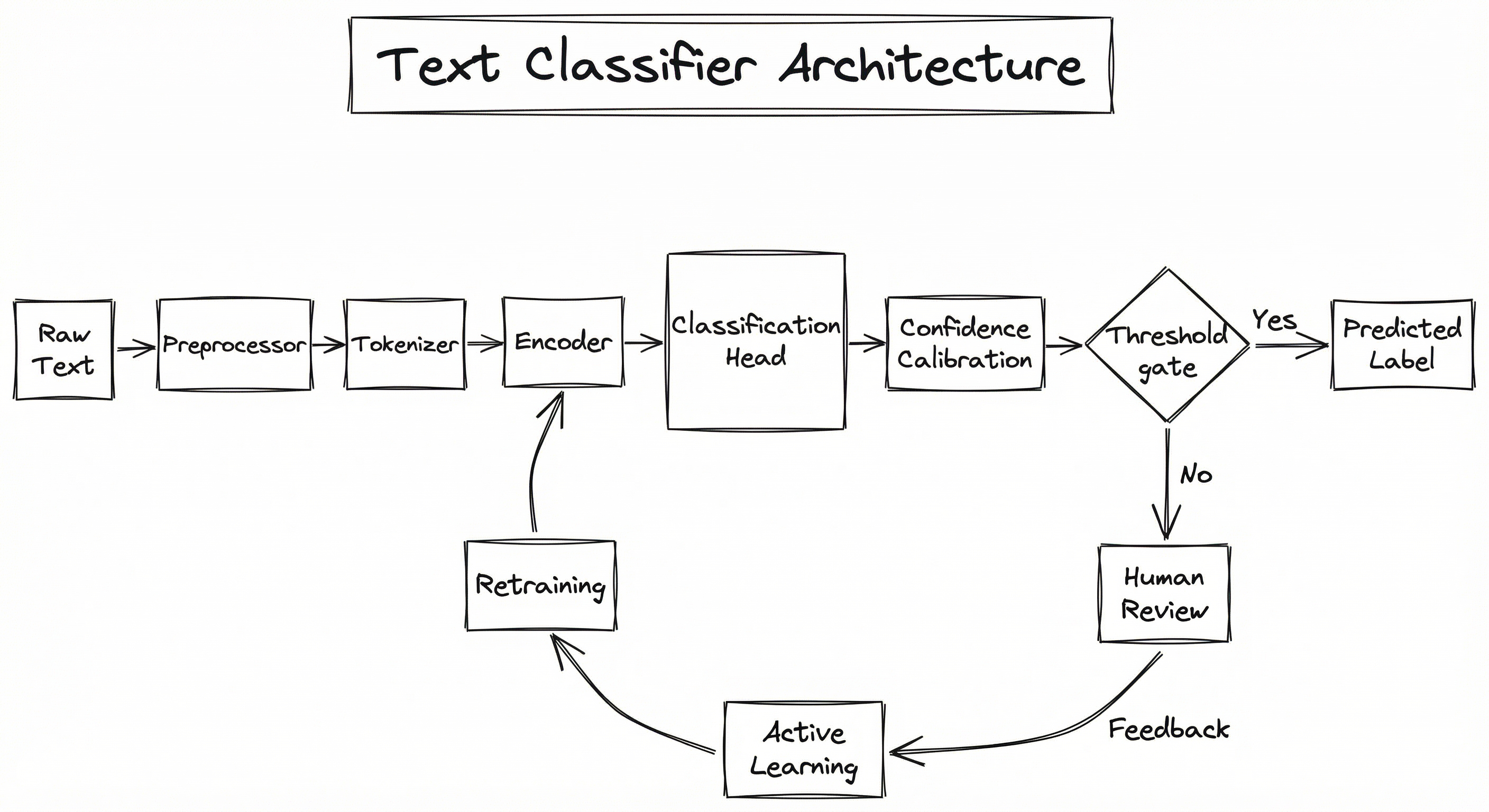
The architecture follows a standard encode-then-classify pattern, but production systems add crucial layers around the core model. The preprocessor normalizes text (lowercasing, URL removal, emoji handling, language detection). The tokenizer converts text to model-consumable tokens. The encoder produces a dense representation -- this could be TF-IDF vectors, a pre-trained BERT model, or sentence embeddings. The classification head maps the representation to label probabilities. Confidence calibration ensures the model's probability outputs are meaningful (a model that says 90% should be right 90% of the time). And the human review queue catches low-confidence predictions for manual labeling, creating a feedback loop that continuously improves the system.
Key Components
Text Preprocessor
Normalizes raw input: lowercasing, stripping HTML, handling emojis and special characters, detecting language, truncating or segmenting overly long texts. For Indian language content, includes script detection and transliteration handling.
Tokenizer
Converts text to model-consumable tokens. For transformer models, uses the model's native tokenizer (WordPiece for BERT, BPE for RoBERTa). For classical models, handles n-gram extraction. Must handle multilingual text for Indian deployments (Devanagari, Tamil, Telugu scripts).
Encoder / Feature Extractor
Produces a fixed-dimensional vector representation of the input text. Options range from sparse TF-IDF vectors to dense transformer embeddings ( for BERT-base). This is the most computationally expensive component.
Classification Head
A lightweight layer (typically one or two linear layers with dropout) that maps the encoder output to label logits. For single-label: softmax activation. For multi-label: independent sigmoids per class.
Confidence Calibrator
Post-hoc calibration (temperature scaling, Platt scaling) to ensure predicted probabilities reflect true likelihoods. Critical for systems that use confidence thresholds to route low-confidence predictions to human review.
Active Learning Selector
Selects the most informative unlabeled samples for human annotation, using strategies like uncertainty sampling, margin sampling, or query-by-committee. Reduces annotation cost by 40-70% compared to random labeling.
Model Registry & A/B Testing
Manages model versions, handles canary deployments, and runs online A/B tests comparing model versions. Ensures safe rollout of model updates without degrading production quality.
Data Flow
Training Path: Raw text corpus -> preprocessor -> tokenizer -> encoder produces embeddings -> classification head trained with cross-entropy loss -> model checkpointed to registry -> evaluation on held-out test set -> deployed if metrics meet threshold.
Inference Path: User text -> preprocessor (same pipeline as training) -> tokenizer -> encoder -> classification head -> softmax/sigmoid -> confidence calibration -> if confidence >= threshold, return label; else route to human review queue.
Feedback Loop: Human-reviewed samples -> added to training set -> active learning selector identifies next batch of informative samples from unlabeled pool -> annotated by human reviewers -> model retrained on expanded dataset.
The training and inference paths share the preprocessing and tokenization components, which is critical -- any mismatch between training and serving preprocessing (known as training-serving skew) will silently degrade model quality.
A directed flow showing Raw Text -> Preprocessor -> Tokenizer -> Encoder -> Classification Head -> Confidence Calibration -> decision gate splitting to Predicted Label (high confidence) or Human Review Queue (low confidence), with a feedback loop from Human Review through Active Learning Selector back to the Retraining Pipeline and Encoder.
How to Implement
Choosing Your Approach
The implementation strategy depends primarily on three factors: (1) how much labeled data you have, (2) your latency budget, and (3) your compute budget. Here's the decision tree:
100K+ labeled examples, latency < 5ms: TF-IDF + Logistic Regression or Linear SVM. Don't laugh -- this is still a strong baseline that's shockingly hard to beat on many tasks. Training takes minutes on a CPU. Inference is microseconds. F1 scores of 0.85-0.90 are common.
1K-100K labeled examples, latency < 50ms: Fine-tuned BERT, DistilBERT, or ModernBERT. The sweet spot for most production systems. Fine-tuning takes 1-4 hours on a single GPU. Inference is 5-20ms on GPU, 30-100ms on CPU with ONNX optimization.
8-64 labeled examples per class: SetFit (Sentence Transformer Fine-Tuning). Remarkably effective with minimal data -- achieves 92.7% accuracy on IMDB with just 8 examples per class. No prompts needed, runs on a single GPU.
Zero labeled examples: Zero-shot classification using NLI models like bart-large-mnli or deberta-v3-base-tasksource-nli. You provide candidate labels as text, and the model determines entailment. Quality varies but is often good enough for prototyping or low-stakes classification.
Massive unlabeled corpus + small labeling budget: Active learning loop. Start with a zero-shot or few-shot model, use uncertainty sampling to select the most informative samples for human labeling, retrain, repeat. Recent research shows this can retain 93% of GPT-4's classification performance at 6% of the cost.
Cost Context (India): Fine-tuning BERT-base on an A100 GPU via E2E Networks costs approximately INR 170/hour (~1.50). Compare this to GPT-4 API calls for the same 50K samples at ~$75 (INR 6,300). The economics heavily favor fine-tuned local models for high-volume classification.
from sklearn.feature_extraction.text import TfidfVectorizer
from sklearn.linear_model import LogisticRegression
from sklearn.pipeline import Pipeline
from sklearn.model_selection import cross_val_score
from sklearn.metrics import classification_report
import numpy as np

# Sample data
texts = [
    "Get rich quick! Buy now!",
    "Meeting scheduled for tomorrow at 3 PM",
    "Congratulations! You won a free iPhone",
    "Please review the attached quarterly report",
    "Limited time offer - 90% discount!!!",
    "Team standup moved to 10 AM",
]
labels = ["spam", "ham", "spam", "ham", "spam", "ham"]

# Build pipeline
pipeline = Pipeline([
    ('tfidf', TfidfVectorizer(
        max_features=50000,
        ngram_range=(1, 3),       # unigrams, bigrams, trigrams
        sublinear_tf=True,         # apply log normalization
        min_df=2,                  # ignore very rare terms
        strip_accents='unicode',
    )),
    ('clf', LogisticRegression(
        C=1.0,
        class_weight='balanced',   # handle class imbalance
        max_iter=1000,
        solver='lbfgs',
    ))
])

# Cross-validation
scores = cross_val_score(pipeline, texts, labels, cv=3, scoring='f1_macro')
print(f"Macro F1: {np.mean(scores):.3f} (+/- {np.std(scores):.3f})")

# Train and evaluate
pipeline.fit(texts, labels)
preds = pipeline.predict(texts)
print(classification_report(labels, preds))
This is the baseline you should always build first. TF-IDF with n-grams captures surface-level patterns remarkably well. sublinear_tf=True applies logarithmic term frequency scaling, which prevents common words from dominating. class_weight='balanced' automatically adjusts for imbalanced classes. On many production tasks (especially with clean, English-only data), this baseline achieves F1 scores of 0.85-0.90 and serves as a strong sanity check before investing in transformer-based approaches.
from transformers import (
    AutoTokenizer,
    AutoModelForSequenceClassification,
    TrainingArguments,
    Trainer,
)
from datasets import load_dataset
import numpy as np
from sklearn.metrics import f1_score, accuracy_score

# Load dataset (example: AG News - 4 topic classes)
dataset = load_dataset("ag_news")
label_names = dataset["train"].features["label"].names  # World, Sports, Business, Sci/Tech

# Load tokenizer and model
model_name = "bert-base-uncased"  # or "answerdotai/ModernBERT-base" for ModernBERT
tokenizer = AutoTokenizer.from_pretrained(model_name)
model = AutoModelForSequenceClassification.from_pretrained(
    model_name,
    num_labels=len(label_names),
    problem_type="single_label_classification",
)

# Tokenize
def tokenize_fn(examples):
    return tokenizer(
        examples["text"],
        padding="max_length",
        truncation=True,
        max_length=256,
    )

tokenized = dataset.map(tokenize_fn, batched=True, remove_columns=["text"])

# Metrics
def compute_metrics(eval_pred):
    logits, labels = eval_pred
    preds = np.argmax(logits, axis=-1)
    return {
        "accuracy": accuracy_score(labels, preds),
        "f1_macro": f1_score(labels, preds, average="macro"),
        "f1_weighted": f1_score(labels, preds, average="weighted"),
    }

# Training arguments
training_args = TrainingArguments(
    output_dir="./results",
    num_train_epochs=3,
    per_device_train_batch_size=32,
    per_device_eval_batch_size=64,
    learning_rate=2e-5,             # standard for BERT fine-tuning
    weight_decay=0.01,
    warmup_ratio=0.1,               # 10% warmup
    eval_strategy="epoch",
    save_strategy="epoch",
    load_best_model_at_end=True,
    metric_for_best_model="f1_macro",
    fp16=True,                       # mixed precision for speed
    logging_steps=100,
    report_to="wandb",               # optional: W&B logging
)

# Train
trainer = Trainer(
    model=model,
    args=training_args,
    train_dataset=tokenized["train"],
    eval_dataset=tokenized["test"],
    compute_metrics=compute_metrics,
)
trainer.train()

# Evaluate
results = trainer.evaluate()
print(f"Test F1 (macro): {results['eval_f1_macro']:.4f}")
This is the standard recipe for fine-tuning BERT (or any transformer) for text classification. Key details: (1) learning rate of 2e-5 is the well-established sweet spot for BERT fine-tuning -- going higher causes catastrophic forgetting, going lower wastes compute. (2) warmup_ratio=0.1 prevents early training instability. (3) fp16=True enables mixed-precision training, cutting memory usage and training time roughly in half. (4) We track f1_macro instead of accuracy because it gives equal weight to all classes, which is critical for imbalanced datasets. On AG News, expect ~94% accuracy after 3 epochs.
from setfit import SetFitModel, Trainer, TrainingArguments, sample_dataset
from datasets import load_dataset
from sklearn.metrics import classification_report

# Load dataset and sample few-shot examples
dataset = load_dataset("SetFit/sst2")  # sentiment: positive/negative
train_dataset = sample_dataset(
    dataset["train"],
    label_column="label",
    num_samples=8,  # only 8 examples per class!
)
eval_dataset = dataset["validation"]

# Initialize SetFit model
model = SetFitModel.from_pretrained(
    "sentence-transformers/paraphrase-MiniLM-L6-v2",
    labels=["negative", "positive"],
)

# Training arguments
args = TrainingArguments(
    batch_size=16,
    num_epochs=1,            # contrastive learning phase
    num_iterations=20,       # number of text pairs per step
    body_learning_rate=1e-5,
    head_learning_rate=1e-2,
)

# Train
trainer = Trainer(
    model=model,
    args=args,
    train_dataset=train_dataset,
    eval_dataset=eval_dataset,
)
trainer.train()

# Evaluate
metrics = trainer.evaluate(eval_dataset)
print(f"Accuracy: {metrics['accuracy']:.4f}")

# Inference
predictions = model.predict([
    "This movie was absolutely fantastic!",
    "Terrible waste of time.",
    "The food was okay, nothing special.",
])
print(predictions)  # ["positive", "negative", "negative"]
SetFit is a game-changer for scenarios where you have very few labeled examples. It works in two phases: (1) contrastive learning -- generates positive and negative text pairs from your few examples and fine-tunes the sentence transformer to push similar texts closer and dissimilar texts apart, (2) classification head training -- trains a logistic regression head on the fine-tuned embeddings. With just 8 examples per class, SetFit achieves 92.7% accuracy on IMDB (compared to 25K examples needed for full fine-tuning). The model is also much smaller than BERT -- paraphrase-MiniLM-L6-v2 is only 80MB.
from transformers import pipeline

# Initialize zero-shot classifier
classifier = pipeline(
    "zero-shot-classification",
    model="facebook/bart-large-mnli",  # or "MoritzLaurer/deberta-v3-large-zeroshot-v2.0"
    device=0,  # GPU
)

# Single-label classification
result = classifier(
    "The new iPhone 16 Pro has an amazing camera system",
    candidate_labels=["technology", "sports", "politics", "entertainment", "business"],
)
print(f"Label: {result['labels'][0]}, Score: {result['scores'][0]:.3f}")
# Label: technology, Score: 0.912

# Multi-label classification
result = classifier(
    "The CEO announced record profits while laying off 500 workers",
    candidate_labels=["business", "employment", "ethics", "finance"],
    multi_label=True,
)
for label, score in zip(result['labels'], result['scores']):
    print(f"{label}: {score:.3f}")
# business: 0.934
# finance: 0.821
# employment: 0.789
# ethics: 0.612

# Multilingual example (Hindi)
result = classifier(
    "प्रधानमंत्री ने नई शिक्षा नीति की घोषणा की",
    candidate_labels=["politics", "education", "sports", "technology"],
)
print(f"Label: {result['labels'][0]}")
# Label: education
Zero-shot classification works by reformulating the task as Natural Language Inference (NLI). For each candidate label, the model evaluates whether the input text (premise) entails a hypothesis like "This text is about {label}." The label with the highest entailment score wins. This requires zero training data -- you just provide candidate labels as strings. The trade-off is lower accuracy compared to fine-tuned models (typically 5-15% lower F1), but it's invaluable for rapid prototyping, label exploration, and scenarios where the label set changes frequently.
import torch
import torch.nn as nn
from transformers import AutoModel, AutoTokenizer

class FocalLoss(nn.Module):
    """Focal loss for handling class imbalance in multi-label classification."""
    def __init__(self, alpha=0.25, gamma=2.0):
        super().__init__()
        self.alpha = alpha
        self.gamma = gamma

    def forward(self, logits, targets):
        bce_loss = nn.functional.binary_cross_entropy_with_logits(
            logits, targets, reduction='none'
        )
        probs = torch.sigmoid(logits)
        p_t = probs * targets + (1 - probs) * (1 - targets)
        focal_weight = self.alpha * (1 - p_t) ** self.gamma
        return (focal_weight * bce_loss).mean()

class MultiLabelClassifier(nn.Module):
    def __init__(self, model_name, num_labels, dropout=0.1):
        super().__init__()
        self.encoder = AutoModel.from_pretrained(model_name)
        hidden_size = self.encoder.config.hidden_size
        self.classifier = nn.Sequential(
            nn.Dropout(dropout),
            nn.Linear(hidden_size, hidden_size // 2),
            nn.GELU(),
            nn.Dropout(dropout),
            nn.Linear(hidden_size // 2, num_labels),
        )
        self.loss_fn = FocalLoss(alpha=0.25, gamma=2.0)

    def forward(self, input_ids, attention_mask, labels=None):
        outputs = self.encoder(input_ids=input_ids, attention_mask=attention_mask)
        cls_output = outputs.last_hidden_state[:, 0, :]  # [CLS] token
        logits = self.classifier(cls_output)

        loss = None
        if labels is not None:
            loss = self.loss_fn(logits, labels.float())

        return {"loss": loss, "logits": logits}

# Usage
tokenizer = AutoTokenizer.from_pretrained("bert-base-uncased")
model = MultiLabelClassifier("bert-base-uncased", num_labels=10)

# Inference
text = "Breaking: Tech giant announces layoffs amid strong quarterly earnings"
inputs = tokenizer(text, return_tensors="pt", padding=True, truncation=True)
with torch.no_grad():
    output = model(**inputs)
    probs = torch.sigmoid(output["logits"])
    # Apply threshold (0.5 default, tune per-class in production)
    predicted_labels = (probs > 0.5).int()
    print(f"Probabilities: {probs}")
    print(f"Predicted labels: {predicted_labels}")
This example demonstrates two critical production patterns: (1) multi-label classification using independent sigmoid activations instead of softmax, allowing a text to belong to multiple categories simultaneously, and (2) focal loss for handling class imbalance. The focal loss with down-weights easy examples by up to 100x, forcing the model to focus on hard-to-classify samples. The two-layer classification head with GELU activation and dropout provides better expressiveness than a single linear layer. In production, you'd tune the classification threshold per-class rather than using a global 0.5 cutoff.
import numpy as np
from sklearn.feature_extraction.text import TfidfVectorizer
from sklearn.linear_model import LogisticRegression
from sklearn.metrics import f1_score

def uncertainty_sampling(model, X_pool, n_samples=50):
    """Select samples where the model is most uncertain (closest to 0.5)."""
    probs = model.predict_proba(X_pool)
    # Entropy-based uncertainty
    entropy = -np.sum(probs * np.log(probs + 1e-10), axis=1)
    uncertain_indices = np.argsort(entropy)[-n_samples:]
    return uncertain_indices

def active_learning_loop(
    X_labeled, y_labeled, X_pool, y_pool_oracle,
    X_test, y_test,
    n_iterations=10, samples_per_iteration=50
):
    """Run an active learning loop with uncertainty sampling."""
    vectorizer = TfidfVectorizer(max_features=10000, ngram_range=(1, 2))
    results = []

    for iteration in range(n_iterations):
        # Fit vectorizer on all available text
        all_text = list(X_labeled) + list(X_pool)
        vectorizer.fit(all_text)

        X_train_vec = vectorizer.transform(X_labeled)
        X_pool_vec = vectorizer.transform(X_pool)
        X_test_vec = vectorizer.transform(X_test)

        # Train model
        model = LogisticRegression(class_weight='balanced', max_iter=1000)
        model.fit(X_train_vec, y_labeled)

        # Evaluate
        preds = model.predict(X_test_vec)
        f1 = f1_score(y_test, preds, average='macro')
        results.append({
            'iteration': iteration,
            'labeled_samples': len(X_labeled),
            'f1_macro': f1
        })
        print(f"Iter {iteration}: {len(X_labeled)} samples, F1={f1:.3f}")

        if len(X_pool) == 0:
            break

        # Select most uncertain samples
        uncertain_idx = uncertainty_sampling(model, X_pool_vec, samples_per_iteration)

        # Simulate human labeling (in production, send to annotation UI)
        X_new = [X_pool[i] for i in uncertain_idx]
        y_new = [y_pool_oracle[i] for i in uncertain_idx]

        # Add to labeled set, remove from pool
        X_labeled = list(X_labeled) + X_new
        y_labeled = list(y_labeled) + y_new
        X_pool = [x for i, x in enumerate(X_pool) if i not in uncertain_idx]
        y_pool_oracle = [y for i, y in enumerate(y_pool_oracle) if i not in uncertain_idx]

    return results

# Example usage
# results = active_learning_loop(X_seed, y_seed, X_unlabeled, y_oracle, X_test, y_test)
Active learning dramatically reduces labeling cost by intelligently selecting which samples to annotate. Instead of randomly labeling 10,000 samples, you might achieve the same F1 score by labeling only 2,000-3,000 samples chosen via uncertainty sampling. The loop works as follows: (1) train on current labeled data, (2) predict on unlabeled pool, (3) select the most uncertain predictions (highest entropy), (4) send those to human annotators, (5) add newly labeled samples and repeat. Research shows this approach can reduce annotation costs by 40-70%. For Indian startups where annotation resources are limited, this is essential.
# Text Classifier Training Configuration (YAML)
model:
  architecture: bert-base-uncased  # or answerdotai/ModernBERT-base
  num_labels: 5
  problem_type: single_label_classification  # or multi_label_classification
  max_seq_length: 256
  dropout: 0.1

training:
  epochs: 3
  batch_size: 32
  learning_rate: 2e-5
  weight_decay: 0.01
  warmup_ratio: 0.1
  fp16: true
  gradient_accumulation_steps: 1
  early_stopping_patience: 3
  metric_for_best_model: f1_macro

data:
  train_path: ./data/train.jsonl
  eval_path: ./data/eval.jsonl
  test_path: ./data/test.jsonl
  text_column: text
  label_column: label
  class_weights: balanced  # or custom: [1.0, 2.5, 1.0, 3.0, 1.0]

serving:
  engine: onnx  # or torchscript, triton
  quantization: int8  # reduces model size 4x, ~5% F1 drop
  confidence_threshold: 0.85
  fallback: human_review
  max_batch_size: 64
  timeout_ms: 100
Common Implementation Mistakes
- ●
Not building a TF-IDF baseline first: Jumping straight to BERT without a simple baseline means you have no way to quantify the value of the extra complexity. I've seen teams spend weeks fine-tuning transformers only to discover that TF-IDF + logistic regression was within 2% F1. Always start simple.
- ●
Ignoring class imbalance: Training on imbalanced data with standard cross-entropy loss produces a model that predicts the majority class for everything. Use
class_weight='balanced', focal loss, or oversampling (SMOTE for tabular features, back-translation or synonym replacement for text augmentation). - ●
Using accuracy as the primary metric for imbalanced datasets: A spam detector that always predicts "not spam" achieves 99% accuracy on a dataset with 1% spam. That's useless. Use F1-score (macro or weighted), precision-recall curves, and AUC-ROC instead.
- ●
Training-serving skew in preprocessing: The preprocessing applied during training must be identical during inference. If you lowercase text during training but forget to during serving, your model sees completely different inputs. Use a shared preprocessing pipeline (or better, let the tokenizer handle everything).
- ●
Overfitting on small datasets without regularization: Fine-tuning BERT on fewer than 1,000 examples without dropout, weight decay, and early stopping almost guarantees overfitting. Watch the gap between training and validation loss closely.
- ●
Not calibrating confidence scores: Raw softmax outputs are not calibrated probabilities. A model that outputs 0.95 for a prediction might only be correct 70% of the time. Apply temperature scaling or Platt scaling if you use confidence thresholds for routing decisions.
- ●
Ignoring label quality: Garbage labels in, garbage model out. Inter-annotator agreement below 0.7 (Cohen's kappa) means your label definitions are ambiguous. Fix the labeling guidelines before blaming the model.
When Should You Use This?
Use When
You need to automatically route, filter, or categorize text at scale -- support tickets, reviews, emails, chat messages, or social media posts
Your label taxonomy is well-defined and reasonably stable (adding new labels is possible but shouldn't happen daily)
You have at least some labeled data (even 8 examples per class suffices with SetFit) or can define labels clearly enough for zero-shot classification
The classification task requires understanding the meaning of text, not just keyword matching -- e.g., detecting sarcastic complaints vs. genuine praise
You need consistent, reproducible categorization that doesn't vary with annotator mood or fatigue
Downstream systems (routing, analytics, alerting) depend on structured labels derived from unstructured text
You're building a content moderation, spam detection, intent detection, or sentiment analysis system
Avoid When
The task is better served by keyword matching or regex -- if "cancel my order" always means cancellation regardless of context, a simple rule is more maintainable and debuggable than a model
Your label taxonomy is unstable and changes weekly -- retraining and redeploying models for every label change is expensive; consider zero-shot approaches or LLM-based classification instead
You need to extract specific entities rather than categorize the whole text -- use NER (named entity recognition) instead
The text is too short to carry meaningful signal (single words, product codes) -- consider structured lookup or fuzzy matching instead
You need generative output (summaries, translations, rewrites) rather than categorical labels -- use a language model instead
The number of classes exceeds 1,000 and data per class is sparse -- consider extreme multi-label classification techniques or hierarchical classification
Key Tradeoffs
The Accuracy-Latency-Cost Triangle
Every text classification system navigates a three-way tradeoff:
| Approach | F1 (typical) | Latency (CPU) | Latency (GPU) | Training Cost | Model Size |
|---|---|---|---|---|---|
| TF-IDF + LR | 0.85-0.90 | <1ms | N/A | Minutes | <100MB |
| DistilBERT | 0.90-0.93 | 30-60ms | 5-10ms | 1-2 hrs | 260MB |
| BERT-base | 0.92-0.95 | 60-120ms | 8-15ms | 2-4 hrs | 440MB |
| ModernBERT | 0.93-0.95 | 40-80ms | 5-10ms | 1-3 hrs | 400MB |
| SetFit (8-shot) | 0.88-0.93 | 5-15ms | 2-5ms | 5-15 min | 80-350MB |
| Zero-shot (BART-MNLI) | 0.75-0.88 | 200-500ms | 20-50ms | 0 | 1.6GB |
When to Use What: A Pragmatic Framework
Start with TF-IDF + LR. Seriously. Train it in 5 minutes, get your baseline number, and use that to decide if you need a transformer at all. If the baseline hits your quality bar, ship it. You'll save thousands in GPU costs.
Graduate to fine-tuned transformers when: (a) the TF-IDF baseline is 5+ percentage points below your target, (b) the text requires deep semantic understanding (sarcasm, context-dependent meaning), or (c) you're working with multilingual text where TF-IDF features don't transfer well.
Use SetFit when you have very few labeled examples but high-quality ones. It's particularly effective for domain-specific tasks where getting labeled data is expensive -- medical text classification, legal document categorization, or specialized technical support ticket routing.
Use zero-shot for prototyping, label exploration, or when the label set changes frequently. It's also useful as a teacher model in a knowledge distillation setup -- use zero-shot to label a large corpus, then train a smaller, faster student model on those labels.
Cost Note: For an Indian startup processing 1M texts/day, the annual compute cost difference between TF-IDF (CPU-only, ~INR 3 lakh/year) and BERT (GPU-required, ~INR 15-25 lakh/year) is significant. Make sure the accuracy improvement justifies the 5-8x cost increase.
Alternatives & Comparisons
Sentiment analysis is a specialized case of text classification where the labels are sentiment polarities (positive, negative, neutral) or emotion categories. If your only goal is sentiment detection, dedicated sentiment models (fine-tuned on sentiment corpora) typically outperform generic classifiers. But if you need sentiment alongside other categories (topic + sentiment), a general text classifier with multi-label output is more flexible.
NER extracts specific spans from text (person names, dates, locations), while text classification assigns whole-document labels. They're complementary, not competing. A support ticket system might use NER to extract the product name and order ID, then use text classification to route the ticket to the right team. Choose NER when you need to find and extract entities; choose classification when you need to categorize the entire text.
An alternative to training a dedicated classifier is to embed texts and use k-NN lookup against a labeled reference set. This is more flexible (new classes can be added by adding reference examples without retraining) but less precise than a fine-tuned classifier. It works well when classes change frequently or when you want a single embedding model serving multiple downstream tasks. The downside is higher inference latency and the need to manage a reference index.
Using a large language model (GPT-4, Claude, Gemini) with prompt engineering for classification is increasingly common. It excels at nuanced, context-heavy tasks and requires no training data -- just a well-crafted prompt. However, it's 100-1000x more expensive per inference than a fine-tuned BERT model, latency is 500ms-5s (vs. 10-50ms), and you're dependent on an external API. Use LLM classification for low-volume, high-stakes tasks; use dedicated classifiers for high-volume production workloads.
Pros, Cons & Tradeoffs
Advantages
Massive speed and cost advantage over manual categorization -- a fine-tuned BERT classifier processes 1,000 texts per second on a single GPU, vs. a human annotator doing 100-200 per hour
Transfer learning dramatically reduces data requirements -- BERT pre-trained on billions of tokens needs only 1K-10K labeled examples to achieve production-quality classification, and SetFit can work with as few as 8 examples per class
Consistent and reproducible -- unlike human annotators, a model applies the same decision boundary every time, eliminating annotator fatigue, bias, and inter-annotator disagreement
Scales from simple to sophisticated -- the same conceptual pipeline (encode text -> classify) works whether you use TF-IDF or a 100B-parameter language model, letting you start simple and upgrade incrementally
Rich ecosystem of pre-trained models -- Hugging Face hosts thousands of pre-trained classifiers for common tasks (sentiment, toxicity, topic, language detection) that can be used directly or fine-tuned further
Multilingual capability -- models like XLM-RoBERTa and multilingual BERT handle 100+ languages in a single model, critical for Indian deployments where user text spans Hindi, Tamil, Telugu, Bengali, and English
Zero-shot and few-shot options provide viable classification even when labeled data is unavailable, enabling rapid prototyping and label exploration
Disadvantages
Requires labeled data for best performance -- while zero-shot works, it typically lags 5-15% behind fine-tuned models; collecting high-quality labeled data is often the bottleneck, not the modeling
Brittle to distribution shift -- a classifier trained on formal English support tickets will struggle with informal Hindi-English code-mixed social media text. Models need periodic retraining as user language evolves
Class imbalance is pervasive -- real-world classification tasks almost always have skewed distributions (99% ham, 1% spam), requiring specialized techniques (focal loss, oversampling, threshold tuning) to handle correctly
Opaque decision-making -- transformer-based classifiers are black boxes; explaining why a specific email was flagged as spam requires additional interpretability tools (LIME, SHAP, attention analysis)
Latency constraints for transformer models -- BERT-base takes 60-120ms on CPU per inference, which may be too slow for real-time applications; requires GPU serving or model distillation for latency-sensitive paths
Label taxonomy maintenance is ongoing work -- as products evolve, new categories emerge and old ones merge; the classifier needs retraining, and historical data may need relabeling
Failure Modes & Debugging
Label leakage in training data
Cause
Training data contains artifacts that correlate with labels but won't be present at inference time. For example, if spam emails in the training set were collected from a specific domain, the model learns to classify by domain rather than content.
Symptoms
Suspiciously high validation metrics (F1 > 0.99) that don't reproduce on fresh production data. Model performance drops dramatically when deployed to a slightly different data source.
Mitigation
Always evaluate on temporally held-out data (train on January-March, test on April). Inspect feature importances -- if the top features are metadata artifacts rather than content words, you have leakage. Use adversarial validation to detect distribution differences between train and test.
Catastrophic forgetting during fine-tuning
Cause
Fine-tuning with a learning rate that's too high or for too many epochs causes the pre-trained model to lose its general language understanding while overfitting to the specific classification task.
Symptoms
Training loss continues to decrease but validation loss increases after 1-2 epochs. Model fails on texts that are linguistically different from the training data despite having the same label.
Mitigation
Use a low learning rate ( for BERT), apply learning rate warmup (10% of training steps), and implement early stopping based on validation F1. Freeze the first N layers for very small datasets (<500 examples). Monitor the gap between training and validation loss.
Distribution shift in production text
Cause
User language, topic distribution, or writing style changes over time. A classifier trained on 2024 customer support tickets may struggle with new product-related issues in 2026. In India, language mixing patterns (Hinglish) evolve rapidly with social media trends.
Symptoms
Gradual decline in classification accuracy, increase in low-confidence predictions routed to human review, rising user complaints about misclassification. Often subtle and detected late.
Mitigation
Monitor classification confidence distributions over time -- a rightward shift in entropy indicates the model is becoming less certain. Implement concept drift detection using statistical tests (PSI, KL-divergence) on feature distributions. Retrain quarterly or when drift is detected.
Adversarial evasion (especially in spam/content moderation)
Cause
Malicious actors deliberately craft text to evade the classifier -- using Unicode homoglyphs (replacing 'a' with Cyrillic 'a'), intentional misspellings, leetspeak, or inserting invisible characters.
Symptoms
Spam or toxic content bypasses the classifier despite the model performing well on standard test sets. New evasion patterns emerge in waves.
Mitigation
Use character-level models or robust tokenizers like RETVec (Google's resilient text vectorizer) that handle adversarial text manipulations. Combine model-based classification with rule-based post-processing for known evasion patterns. Google achieved a 38% improvement in Gmail spam detection by switching to RETVec.
Multi-label threshold miscalibration
Cause
Using a fixed 0.5 threshold for all labels in multi-label classification, when optimal thresholds vary significantly across classes due to different base rates and class difficulties.
Symptoms
Some labels are over-predicted (low precision) while others are under-predicted (low recall). Global F1 looks acceptable but per-class metrics reveal severe imbalances.
Mitigation
Tune classification thresholds independently per class using the validation set. Use precision-recall curves to find the optimal threshold for each label based on your precision-recall preference. In production, store thresholds in configuration so they can be adjusted without model retraining.
Tokenizer mismatch or truncation
Cause
Input text exceeds the model's maximum sequence length (512 tokens for BERT, 8192 for ModernBERT) and is silently truncated, potentially removing the most informative part of the text.
Symptoms
Model performs well on short texts but poorly on long documents. Classification quality appears to degrade randomly on longer inputs.
Mitigation
Analyze your text length distribution before choosing a model. If most texts exceed 512 tokens, use ModernBERT (8192 tokens) or implement a chunking strategy: split long documents into overlapping windows, classify each chunk, and aggregate predictions (majority vote or max-confidence). For email classification, consider extracting subject + first paragraph rather than processing the entire body.
Placement in an ML System
Where Does Text Classification Sit in the Pipeline?
Text classification is typically one of the first NLP processing steps applied after basic text preprocessing. It acts as a routing and labeling layer that structures unstructured text for downstream consumption.
In a customer support system (think Freshdesk, Zendesk, or Swiggy's internal tools), the text classifier sits at the entry point: incoming messages are classified by intent (complaint, question, feedback, request) and topic (delivery, payment, product, account), then routed to the appropriate team or automated workflow.
In a content moderation pipeline (social media platforms, e-commerce reviews), the classifier operates as a first-pass filter: texts flagged as potentially toxic, spam, or policy-violating are routed to human moderators, while clearly benign content passes through.
In a RAG pipeline, text classification can serve as a pre-retrieval filter: classify the user's query intent to determine which knowledge base or retrieval strategy to use (e.g., factual questions go to document retrieval, chit-chat goes to a conversational model).
The text classifier is often upstream of more expensive NLP operations like NER, summarization, or generation. By filtering and routing early, it prevents wasted compute on irrelevant texts.
Key Insight: Think of text classification as the traffic cop of your NLP pipeline. It doesn't generate content or extract entities -- it decides where text goes and what happens to it next.
Pipeline Stage
Inference / Serving
Upstream
- tokenizer
- embedding-model
Downstream
- sentiment-analyzer
- ner-extractor
- summarizer
Scaling Bottlenecks
The primary bottleneck is inference throughput vs. latency. A BERT-base model on CPU handles ~30-50 requests/second with 60-120ms latency per request. At Flipkart scale (millions of reviews per day), that's nowhere near enough.
Scaling strategies, in order of implementation complexity:
- Batch inference: Group requests and process in batches of 32-64 on GPU. Improves throughput 10-20x.
- Model distillation: Train a smaller DistilBERT student from your fine-tuned BERT teacher. 40% smaller, 60% faster, typically <1% F1 loss.
- ONNX Runtime / TensorRT: Export to optimized inference formats. 2-4x speedup over vanilla PyTorch.
- INT8 quantization: Reduce model weights from FP32 to INT8. 4x size reduction, 2-3x inference speedup, typically <2% F1 loss.
- Horizontal scaling: Run multiple model replicas behind a load balancer. Linear throughput scaling.
At very high scale (>10M classifications/day), consider a tiered architecture: fast TF-IDF model handles easy cases (high-confidence predictions), transformer model handles only the ambiguous cases routed by the first tier. This can reduce GPU costs by 60-80%.
Production Case Studies
Google replaced Gmail's spam classifier text vectorizer with RETVec (Resilient and Efficient Text Vectorizer), a character-level model specifically designed to handle adversarial text manipulations common in spam. RETVec operates on UTF-8 byte sequences rather than word tokens, making it robust against homoglyph attacks, invisible characters, and intentional misspellings that defeat traditional tokenizers.
38% improvement in spam detection rate, 19.4% reduction in false positives, and 83% reduction in TPU usage -- a rare win on all three axes (quality, safety, cost) simultaneously. The model was open-sourced.
Walmart built a context-aware intent classifier for their voice shopping assistant. The system uses Bi-LSTM and GRU with BERT embeddings to classify user utterances into intents (add-to-cart, search, navigate), incorporating conversation history to resolve ambiguous queries. About 40% of user interactions required contextual understanding.
Achieved 90% accuracy on contextual interactions and 87.68% overall accuracy. The system handles the two most common interactions -- adding products to cart and searching -- which account for 98% of contextual queries.
Flipkart uses text classification extensively for product review categorization across 15+ Indian languages, product cataloging from seller descriptions, and customer query routing. The challenge is uniquely Indian: reviews arrive in Hindi, Tamil, Telugu, Bengali, Kannada, and English (plus code-mixed Hinglish), requiring multilingual classification capabilities.
ML-based classification enabled automated processing of millions of reviews and support tickets daily, reducing manual categorization costs and improving response times. Product categorization accuracy improvements directly impacted search relevance and GMV.
Twitter (now X) developed a topic classification system for tweets, addressing the unique challenge of very short, informal, context-dependent text. The system handles 6,000+ tweets per second, classifying them into topics for trending detection, content recommendations, and content moderation. The research introduced a benchmark with 19 topic categories across 6 domains.
The topic classification system powers Twitter's trending topics, content recommendations, and safety features, processing billions of tweets daily with sub-second classification latency.
Grammarly developed a novel approach to grammatical error correction (GEC) called 'Tag, Not Rewrite' — instead of generating corrected text with a seq2seq model, they frame GEC as a sequence tagging problem where each token receives an edit tag (KEEP, DELETE, REPLACE_with_X, APPEND_X). The GECToR model uses a pre-trained BERT encoder with a linear tag classifier, achieving state-of-the-art accuracy with 10x faster inference than generative approaches (2021).
The tagging approach achieved state-of-the-art results on the BEA-2019 benchmark while being 10x faster than seq2seq models, making it practical for real-time suggestions. This architecture became the foundation for Grammarly's production grammar checking, serving 30M+ daily active users.
Brex built a mostly automated merchant classification system for corporate credit card transactions. With thousands of merchant categories and limited labeled data, they combined weak supervision (Snark labeling functions based on MCC codes and merchant name patterns) with text classification using fine-tuned transformers on merchant names and transaction descriptions. The system handles edge cases like ambiguous merchants (e.g., a gas station that's also a convenience store) (2021).
The automated classifier achieves 92% accuracy across thousands of merchant categories, reducing manual review needs by 80%. The weak supervision approach enabled rapid scaling without requiring massive labeled datasets, making expense categorization seamless for Brex's corporate card users.
Tooling & Ecosystem
The de facto standard library for transformer-based text classification. Provides AutoModelForSequenceClassification, the Trainer API, and the pipeline('text-classification') interface. Supports BERT, RoBERTa, DeBERTa, ModernBERT, and 100+ other architectures out of the box.
Efficient few-shot text classification framework by Hugging Face. Fine-tunes sentence transformers using contrastive learning with as few as 8 labeled examples per class. Achieves 92.7% accuracy on IMDB with 8-shot training, approaching full-data performance.
The baseline toolkit for text classification. TfidfVectorizer + LogisticRegression or LinearSVC is the strongest non-neural baseline. Also provides GridSearchCV, cross_val_score, and classification_report for evaluation.
spaCy's built-in text classification component that integrates into spaCy NLP pipelines. Supports both single-label and multi-label classification. Good for production systems already using spaCy for other NLP tasks (tokenization, NER).
Facebook's lightweight text classification library. Extremely fast training (seconds on millions of examples) and inference (<1ms). Uses sub-word features, making it robust to misspellings. Ideal for high-throughput, latency-critical production systems.
Open-source data labeling platform with built-in active learning support. Provides annotation UI for text classification tasks, integrates with ML backends for pre-annotation and uncertainty sampling, and exports in standard formats compatible with Hugging Face datasets.
Data-centric AI library for finding and fixing label errors in classification datasets. Uses confident learning to detect mislabeled examples. Studies show that 3-10% of benchmark datasets contain label errors; cleaning them often improves model quality more than architecture changes.
High-performance inference engine for deploying trained models. Export PyTorch/TensorFlow models to ONNX format for 2-4x inference speedup. Supports INT8 quantization and GPU/CPU optimization. Essential for serving transformer classifiers at scale.
Research & References
Devlin, Chang, Lee & Toutanova (2019)NAACL 2019
Introduced the pre-train then fine-tune paradigm that revolutionized text classification. BERT's bidirectional self-attention and [CLS] token representation became the standard architecture for sequence classification.
Sun, Qiu, Xu & Huang (2019)CCL 2019
Systematic study of BERT fine-tuning strategies for text classification. Found that learning rate warmup, gradual unfreezing, and task-specific preprocessing significantly impact performance. The go-to reference for BERT fine-tuning recipes.
Tunstall, Reimers, Jo, Bates, Korat, Wasserblat & Pereg (2022)arXiv preprint
Proposed SetFit: contrastive fine-tuning of sentence transformers for few-shot classification. Outperforms GPT-3 on few-shot benchmarks while using 1000x fewer parameters. Achieved near full-data performance with only 8 labeled examples per class.
Lin, Goyal, Girshick, He & Dollar (2017)ICCV 2017
Introduced focal loss to address extreme class imbalance by down-weighting easy examples. Originally for object detection but widely adopted in text classification, especially for spam detection and content moderation where positive class prevalence is <5%.
Yin, Hay & Roth (2019)EMNLP 2019
Formalized zero-shot text classification as an NLI entailment problem. Showed that pre-trained NLI models can classify texts into unseen categories by evaluating entailment between the text (premise) and label descriptions (hypothesis).
Warner, Clavie, et al. (2024)arXiv preprint
Introduced ModernBERT with 8192-token context length, rotary positional embeddings, and Flash Attention. Achieves state-of-the-art on classification benchmarks while being 2-4x faster than BERT. Positioned as a drop-in replacement for BERT-base and BERT-large.
Elie Bursztein et al. (2023)NeurIPS 2023 (Industry Track)
Proposed RETVec, a resilient text vectorizer operating on UTF-8 bytes to defend against adversarial text manipulation in spam classifiers. Deployed in Gmail, achieving 38% better spam detection and 83% reduction in TPU usage.
Ein-Dor, Halfon, Gera, et al. (2020)EMNLP 2020 Findings
Comprehensive study of active learning strategies for text classification. Showed that uncertainty-based sampling reduces labeling cost by 40-70% compared to random selection while maintaining equivalent model quality.
Interview & Evaluation Perspective
Common Interview Questions
- ●
How would you design a text classification system for customer support ticket routing at Swiggy scale (500K+ tickets/day)?
- ●
You have 50 labeled examples per class and need 90% F1. What approach do you take?
- ●
How do you handle class imbalance when 99% of emails are legitimate and 1% are spam?
- ●
Compare TF-IDF + Logistic Regression vs. fine-tuned BERT for text classification. When would you prefer each?
- ●
How would you implement a multi-label classifier where a single product review can have tags for quality, price, delivery, and packaging?
- ●
Your text classifier's F1 has dropped from 0.93 to 0.87 over the past three months. How do you diagnose and fix this?
- ●
How do you handle multilingual text classification for an Indian e-commerce platform where reviews come in 15+ languages?
Key Points to Mention
- ●
Always build and report a TF-IDF baseline before proposing a transformer approach. Interviewers want to see you can calibrate the value of complexity.
- ●
F1-score (macro or weighted), not accuracy, is the right metric for most real-world classification tasks due to class imbalance. Precision vs. recall priority depends on the business context.
- ●
Focal loss with is the standard solution for extreme class imbalance. Mention it alongside class-weighted loss and oversampling as a three-pronged strategy.
- ●
SetFit achieves near-BERT performance with 8 examples per class -- this is a powerful talking point when discussing data-scarce scenarios. Mention it along with zero-shot NLI classification.
- ●
Active learning reduces labeling costs by 40-70% by selecting the most informative samples for annotation instead of random labeling. This shows systems thinking about cost.
- ●
Training-serving skew is the #1 silent killer of classifier quality in production. Identical preprocessing pipelines between training and serving are mandatory.
- ●
Confidence calibration and human-in-the-loop fallback are essential for production systems. Models should know when they don't know.
Pitfalls to Avoid
- ●
Proposing a complex transformer architecture without first establishing that a simpler baseline is insufficient -- this signals that you're chasing complexity rather than solving the problem
- ●
Using accuracy as the evaluation metric for imbalanced datasets -- this is an immediate red flag for interviewers
- ●
Ignoring the data labeling problem -- most classification projects fail not because of bad models but because of bad labels, insufficient labels, or drifting label definitions
- ●
Not discussing deployment and latency -- a model that takes 2 seconds per inference is useless for real-time classification, regardless of its F1 score
- ●
Treating text classification as a one-time model training rather than an ongoing system with monitoring, retraining, and feedback loops
Senior-Level Expectation
A senior/staff engineer should discuss the full lifecycle: data collection and labeling strategy (active learning, label quality audits with Cleanlab), model selection with quantitative justification (not just 'I'd use BERT'), handling of edge cases (multilingual text, adversarial inputs, very long documents), deployment considerations (ONNX optimization, INT8 quantization, batched inference, tiered architecture), monitoring and alerting (confidence distribution drift, per-class F1 tracking, A/B testing new models), and cost optimization (GPU vs. CPU serving, tiered classification with fast-model-first routing). The ability to reason about the data flywheel -- how human review of low-confidence predictions generates training data that improves the model, which reduces the volume sent to human review -- is what separates systems thinkers from model builders.
Summary
Text classification is the foundational NLP task of assigning categorical labels to text -- and despite its conceptual simplicity, building a production text classifier that's accurate, fast, fair, and robust is a genuine systems engineering challenge.
The modern practitioner's toolbox spans a remarkable range: from TF-IDF + logistic regression (still a strong baseline that trains in minutes on CPU) through fine-tuned transformers like BERT and ModernBERT (the accuracy sweet spot for most production systems), to SetFit for few-shot scenarios (92.7% accuracy with just 8 examples per class) and zero-shot NLI classifiers for when you have no labeled data at all. The choice between these approaches is driven by three factors: how much labeled data you have, your latency budget, and your compute budget. Start with the simplest approach that meets your quality bar, and only add complexity when you have evidence it's needed.
Beyond the model itself, production text classification demands attention to class imbalance (focal loss, balanced class weights), evaluation metrics (F1-score, never accuracy alone), confidence calibration (temperature scaling for threshold-based routing), multilingual handling (critical for Indian deployments), adversarial robustness (especially for spam and content moderation), and continuous monitoring for distribution drift. The real competitive advantage isn't in the model architecture -- it's in the data flywheel: a system where low-confidence predictions are routed to human review, generating labeled data that improves the model, which reduces the volume sent to human review, creating a virtuous cycle of ever-improving classification quality at decreasing marginal cost.