Dimensionality Reduction: PCA, LDA, TSNE

In machine learning, features or dimensions are individual independent variables that act as inputs in your system. While making the predictions, models use such features to make the predictions, for instance, if we consider a dataset of houses, the dimensions could include the house's price, size, number of bedrooms, location, and so on. The number of features or dimensions used for modeling a machine-learning algorithm depends on how perfectly they can capture the essence of the problem. With more dimensions come the problem of the Curse Of Dimensionality, high-dimensional datasets pose several practical concerns for machine learning algorithms, such as increased computation time, and storage space for big data, high-dimensional data is hard to visualize, making exploratory data analysis more difficult. etc. However, the biggest concern is perhaps decreased accuracy in predictive models. Statistical and machine learning models trained on high-dimensional datasets often generalize poorly.

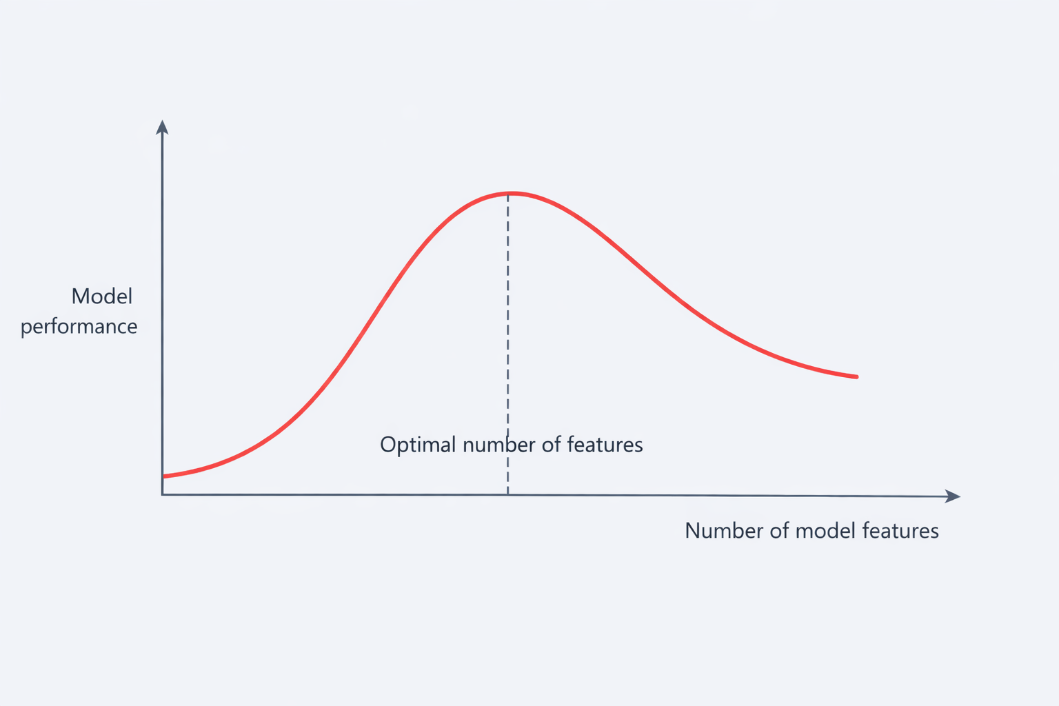
So what do we do to solve this problem….?

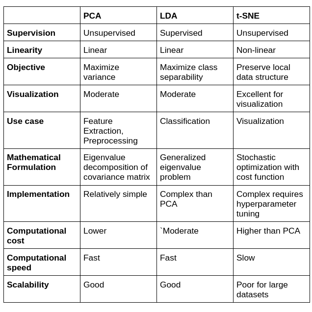
Here comes the technique of Dimensionality Reduction. Dimensionality reduction is a technique used to reduce the number of features in a dataset while retaining as much of the important information as possible. In other words, it is a process of transforming high-dimensional data into a lower-dimensional space that still preserves the essence of the original data. There are several techniques for dimensionality reduction, including principal component analysis (PCA), linear discriminant analysis (LDA), and t-Distributed Stochastic Neighbor Embedding (t-SNE).

Let's go deep into these Dimensionality reduction techniques, where we use them and what is the nitty-gritty behind it.

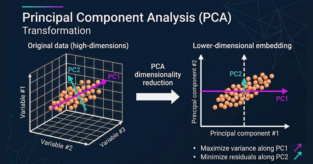
Principal Component Analysis(PCA)

PCA(Principal Component Analysis) is a linear transformation algorithm that seeks to project the original features of our data onto a smaller set of features ( or subspace ) while still retaining most of the information. To do this the algorithm tries to find the most appropriate directions/angles ( which are the principal components ) that maximize the variance in the new subspace. In a nutshell, PCA is an act of finding a new axis to represent the data so that a few principal components may contain the most information. When going from a high-dimensional space(d) to a low-dimensional space (d’ ), preserve dimensions that have high variance (or high / information.)

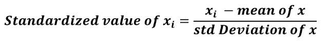
Step 1: Standardize each column

The reason why standardization is very much needed before performing PCA is that PCA is very sensitive to variances. Meaning, if there are large differences between the scales (ranges) of the original variables, then those with larger scales will dominate over those with small scales. Data standardization is the transformation of features by subtracting from the mean and dividing by standard deviation.

‍Step 2: Compute Covariance Matrix

This step aims to understand how the original variables of the input data set vary from the mean concerning each other, or in other words, to see if there is any relationship between them. Because sometimes, original variables are highly correlated in such a way that they contain redundant information. So, to identify these correlations, we compute the covariance matrix.

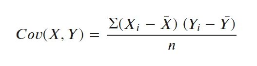
Covariance Matrix

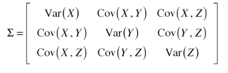
The sign of the variables in the matrix tells us whether combinations are correlated:

• Positive (the original variables are correlated and increase or decrease at the same time)
• Negative (the original variables are not correlated, meaning that one decreases while the other increases)
• Zero (the original variables are not related to each other)
  

Step 3: Compute Eigenvalues and Eigenvectors of Covariance Matrix to Identify Principal Components

Here, we calculate the eigenvectors (principal components) and eigenvalues of the covariance matrix. As eigenvectors, the principal components represent the directions of maximum variance in the data. The eigenvalues represent the amount of variance in each component. Ranking the eigenvectors by eigenvalue identifies the order of principal components. PCA aims to preserve the Euclidean distances between points as much as possible when reducing dimensionality

Step 4: Select the principal components

Here, we decide which components to keep and which to discard. Components with low eigenvalues typically will not be as significant. Scree plots usually plot the proportion of total variance explained and the cumulative proportion of variance. These metrics help one to determine the optimal number of components to retain. The point at which the Y axis of eigenvalues or total variance explained creates an "elbow" will generally indicate how many PCA components we want to include.

Step 5: Transform the data into the new coordinate system

Finally, the data is transformed into the new coordinate system defined by the principal components. That is, the feature vector created from the eigenvectors of the covariance matrix projects the data onto the new axes defined by the principal components. This creates new data, capturing most of the information but with fewer dimensions than the original dataset.

Here are some drawbacks of PCA:

• PCA works only if the observed variables are linearly correlated. If there's no correlation, PCA will fail to capture adequate variance with fewer components.
• PCA is lossy. Information is lost when we discard insignificant components.
• Scaling of variables can yield different results. Hence, the scaling that you use should be documented. Scaling should not be adjusted to match prior knowledge of data.
• Since each principal component is a linear combination of the original features, visualizations are not easy to interpret or relate to original space(features).
  

Real-World Applications of PCA

1. Image Compression: PCA can reduce image size while maintaining key visual information.
2. Finance: PCA is used in risk management and portfolio optimization.
3. Bioinformatics: PCA can identify patterns across thousands of genes in gene expression analysis.
4. Neuroscience: PCA helps analyze complex neural data and understand brain activity patterns.

Implementation of PCA on wine dataset

Here we are using the Wine dataset from the UCI Machine Learning Repository. This dataset contains chemical analysis results of wines grown in the same region in Italy but derived from three different cultivars. It has 13 features, making it suitable for demonstrating the effect of PCA on high-dimensional data.

1. Here we visualize the original space using the first two features.
2. Apply PCA to reduce the dataset to 2 dimensions.
3. Visualize the dataset after applying PCA.
4. Plot both visualizations side by side.
   

import numpy as np
import pandas as pd
import matplotlib.pyplot as plt
from sklearn.decomposition import PCA
from sklearn.datasets import load_wine

# Load the Wine dataset
wine = load_wine()
X = wine.data
y = wine.target

# Convert to DataFrame for better visualization
df = pd.DataFrame(X, columns=wine.feature_names)
df['class'] = y
df['class'] = df['class'].map({0: wine.target_names[0], 1: wine.target_names[1], 2: wine.target_names[2]})

# Plotting the original dataset
plt.figure(figsize=(12, 6))
plt.subplot(1, 2, 1)
for class_label in wine.target_names:    
    subset = df[df['class'] == class_label]
   plt.scatter(subset.iloc[:, 0], subset.iloc[:, 1], label=class_label)
plt.xlabel(wine.feature_names[0])
plt.ylabel(wine.feature_names[1])
plt.title('Original Wine Dataset')
plt.legend()

# Apply PCA
pca = PCA(n_components=2)
X_pca = pca.fit_transform(X)

# Create a DataFrame for the PCA results
df_pca = pd.DataFrame(X_pca, columns=['Principal Component 1', 'Principal Component 2'])
df_pca['class'] = y
df_pca['class'] = df_pca['class'].map({0: wine.target_names[0], 1: wine.target_names[1], 2: wine.target_names[2]})

# Plotting the PCA-transformed dataset
plt.subplot(1, 2, 2)
for class_label in wine.target_names:
   subset = df_pca[df_pca['class'] == class_label]
   plt.scatter(subset['Principal Component 1'], subset['Principal Component 2'], label=class_label)
plt.xlabel('Principal Component 1')
plt.ylabel('Principal Component 2')
plt.title('PCA of Wine Dataset')
plt.legend()
plt.tight_layout()
plt.show()

Here is the comparison of scatter plots of original variables and variables after PCA.

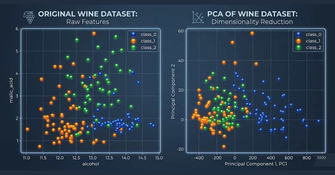
PCA helps in reducing the dimensionality of the dataset while preserving as much variance as possible, making it easier to visualize the data.

PCA and Unsupervised Neural Networks: A Hidden Connection

The relationship between PCA and neural networks is complex, but it’s fascinating to discover that they are related. More specially, PCA can be understood as a type of unsupervised neural network known as an autoencoder when certain conditions prevail.

Autoencoders

An autoencoder is a type of artificial neural network used for unsupervised learning of efficient codings. Autoencoders are architectures that compress the learned representation of the data in neural networks. They comprise an encoder and a decoder whose function is to equip the input data with low-dimensional latent space that captures all important features. Here, the decoder tries to construct the original data from this compressed representation.

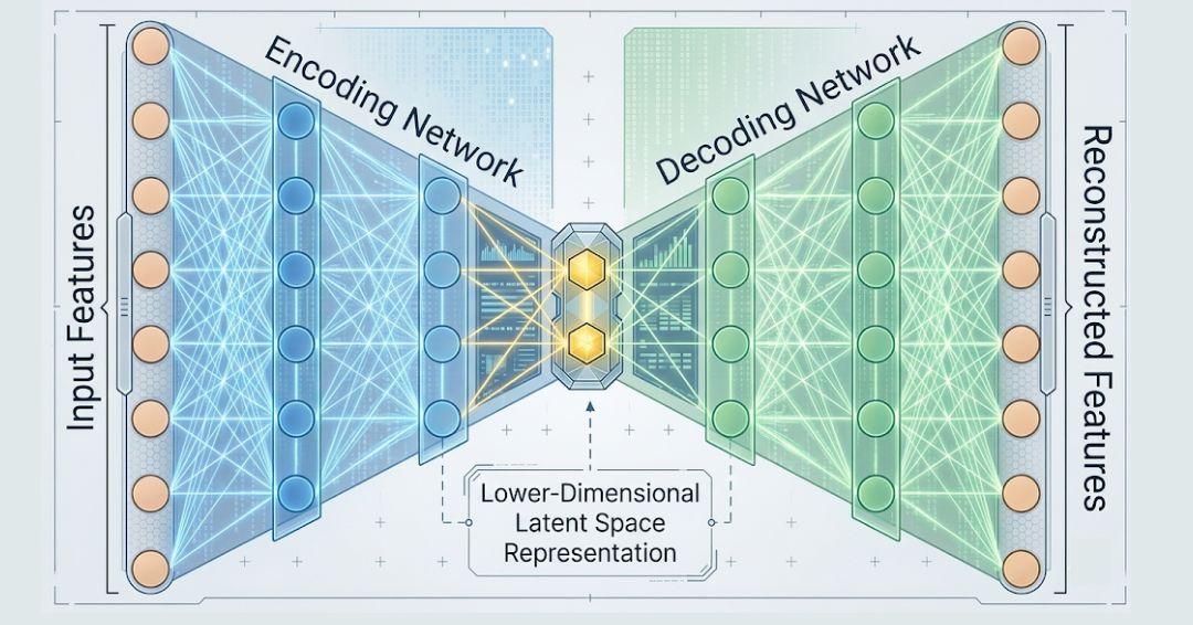
The Key Connection:

For instance, when the loss function used for learning is a mean squared error (MSE), and if it has linear decoders, autoencoders exhibit some characteristics similar to those of PCA. Thus in this particular situation, an autoencoder via training learns how to encode data on a hyperplane equivalent to that employed by PCA!

In both methods, this link demonstrates their basic principles at work. By looking for directions along which there is the highest variability in data, PCA performs dimensional reduction. Similarly, with MSE loss and linear decoder, an autoencoder finds ways to squeeze out valuable information during reconstruction

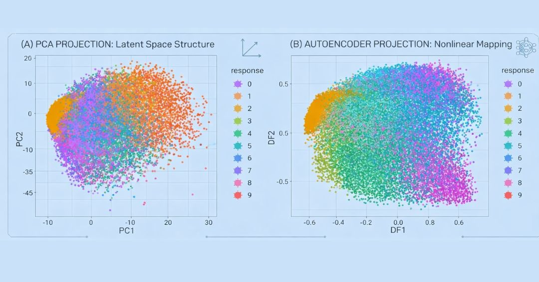
MNIST response variable projected onto a reduced feature space containing only two dimensions. PCA (left) forces a linear projection whereas an autoencoder with non-linear activation functions allows a non-linear project.

Comparison

1. PCA is essentially a linear transformation but Auto-encoders are capable of modeling complex non-linear functions.
2. PCA features are totally linearly uncorrelated with each other since features are projections on an orthogonal basis. However autoencoded features might have correlations since they are just trained for accurate reconstruction.
3. PCA is faster and computationally cheaper than autoencoders.
4. A single-layered autoencoder with a linear activation function is very similar to PCA.
5. Autoencoder is prone to overfitting due to the high number of parameters. (though regularization and careful design can avoid this).
   

Linear Discriminant Analysis(LDA)

Linear Discriminant Analysis (LDA), also known as Normal Discriminant Analysis or Discriminant Function Analysis, is a dimensionality reduction technique primarily utilized in supervised classification problems. It facilitates modeling distinctions between groups, effectively separating two or more classes. LDA operates by projecting features from a higher-dimensional space into a lower-dimensional one.

LDA is like PCA which helps in dimensionality reduction, however, it focuses on maximizing the separability among known categories by creating a new linear axis and projecting the data points on that axis.

‍
Assumptions of LDA

There are some constraints to bear in mind, as the model assumes the following:

1. The input dataset has a Gaussian distribution, where plotting the data points gives a bell-shaped curve.
2. The data set is linearly separable, meaning LDA can draw a straight line or a decision boundary that separates the data points.
3. Each class has the same covariance matrix. 

For these reasons, LDA may not perform well in high-dimensional feature spaces. 

How Does LDA Work?

LDA focuses primarily on projecting the features in higher dimension space to lower dimensions. You can achieve this in three steps:

• Firstly, you need to calculate the separability between classes which is the distance between the mean of different classes. This is called the between-class variance.

• Secondly, calculate the distance between the mean and sample of each class. It is also called the within-class variance.

• Finally, construct the lower-dimensional space which maximizes the between-class variance and minimizes the within-class variance. P is considered as the lower-dimensional space projection, also called Fisher’s criterion.

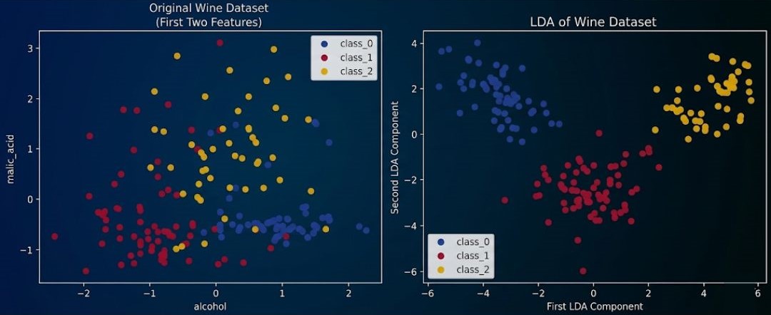
Implementation of LDA on wine dataset

import numpy as np
import pandas as pd
import matplotlib.pyplot as plt
from sklearn.discriminant_analysis import LinearDiscriminantAnalysis as LDA
from sklearn.datasets import load_winefrom sklearn.preprocessing
import StandardScaler

# Load the Wine dataset
wine = load_wine()
X = wine.datay = wine.target

# Standardize the features
scaler = StandardScaler()
X_scaled = scaler.fit_transform(X)

# Apply LDA
lda = LDA(n_components=2)
X_lda = lda.fit_transform(X_scaled, y)

# Plotting
plt.figure(figsize=(12, 5))

# Original data (first two features)
plt.subplot(1, 2, 1)
for i, class_label in enumerate(wine.target_names):  
    mask = y == i  
    plt.scatter(X_scaled[mask, 0], X_scaled[mask, 1], label=class_label)
plt.xlabel(wine.feature_names[0])
plt.ylabel(wine.feature_names[1])
plt.title('Original Wine Dataset\n(First Two Features)')
plt.legend()

# LDA
plt.subplot(1, 2, 2)
for i, class_label in enumerate(wine.target_names):  
    mask = y == i  
   plt.scatter(X_lda[mask, 0], X_lda[mask, 1], label=class_label)
plt.xlabel('First LDA Component')
plt.ylabel('Second LDA Component')
plt.title('LDA of Wine Dataset')
plt.legend()plt.tight_layout()plt.show()

# Print LDA explained variance ratio
print("LDA explained variance ratio:", lda.explained_variance_ratio_)

LDA explained variance ratio: [0.68747889 0.31252111].

The LDA-explained variance ratio is a measure that indicates how much of the variance in the data is explained by each Linear Discriminant Analysis (LDA) component. It's similar to the concept of explained variance ratio in Principal Component Analysis (PCA) but with an important difference.

Real-world Applications of LDA

• Face Recognition – Linear Discriminant Analysis is used in face recognition to reduce the number of attributes to a more manageable number before the actual classification. The dimensions that are generated are a linear combination of pixels that form a template. These are called Fisher’s faces.
• Medical – You can use Linear Discriminant Analysis to classify the patient disease as mild, moderate or severe. The classification is done upon the various parameters of the patient and his medical trajectory. 
• Customer Identification – You can obtain the features of customers by performing a simple question-and-answer survey. Linear Discriminant Analysis helps in identifying and selecting which describes the properties of a group of customers who are most likely to buy a particular item in a shopping mall. 

T-Distributed Stochastic Neighbour Embedding (T-SNE)

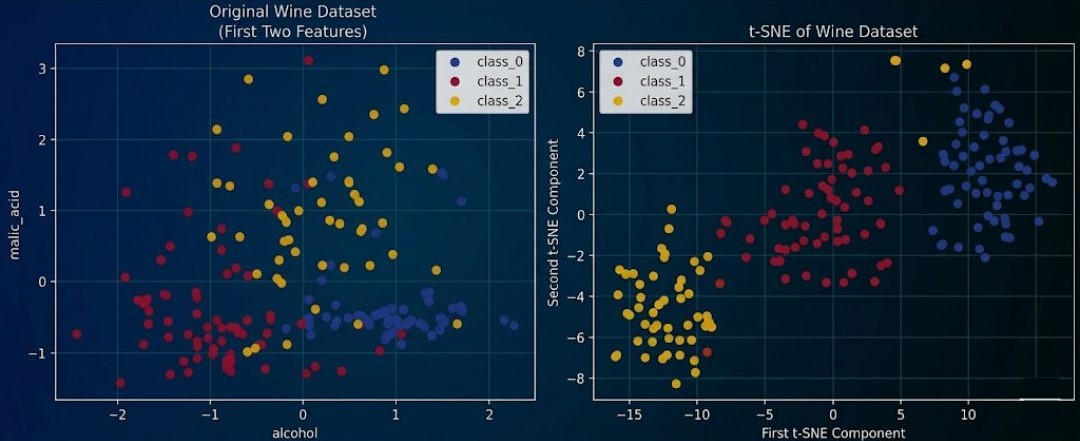
t-Distributed Stochastic Neighbor Embedding (t-SNE algorithm) is a technique for dimensionality reduction that is particularly well suited for visualizing of high-dimensional datasets. t-SNE is a Non-linear Dimensionality reduction technique, which means the algorithm allows us to separate data that a straight line cannot separate.

How t-SNE works

The t-SNE algorithm finds the similarity measure between pairs of instances in higher and lower dimensional space. After that, it tries to optimize two similarity measures. It does all of that in three steps. 

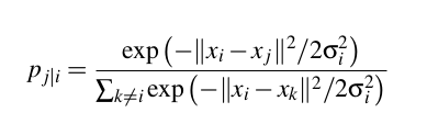
1. t-SNE models a point being selected as a neighbor of another point in both higher and lower dimensions. It starts by calculating a pairwise similarity between all data points in the high-dimensional space using a Gaussian kernel. It uses a T-test from the T-distribution( Student's t distribution is a continuous probability distribution that generalizes the standard normal distribution.). The points that are far apart have a lower probability of being picked than the points that are close together.

             In higher dimensional space:

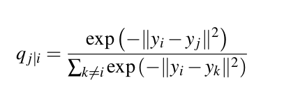
2. Then, the algorithm tries to map higher dimensional data points onto low dimensional space while preserving the pairwise similarities. 

              In lower dimensional space:

3. It is achieved by minimizing the divergence between the probability distribution of the original high-dimensional space and the low-dimensional space. The algorithm uses gradient descent to minimize the divergence. The lower-dimensional embedding is optimized to a stable state.

T-SNE minimizes the sum of KL divergences over all the data points.

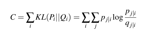
The optimization process allows the creation of clusters and sub-clusters of similar data points in the lower-dimensional space that are visualized to understand the structure and relationship in the higher-dimensional data. 

Implementation of t-SNE on wine dataset

import numpy as np
import pandas as pd
import matplotlib.pyplot as plt
from sklearn.manifold import TSNE
from sklearn.datasets import load_wine
from sklearn.preprocessing import StandardScaler

# Load the Wine dataset
wine = load_wine()
X = wine.data
y = wine.target

# Standardize the features
scaler = StandardScaler()
X_scaled = scaler.fit_transform(X)

# Apply t-SNE
tsne = TSNE(n_components=2, random_state=42)
X_tsne = tsne.fit_transform(X_scaled)

# Plotting
plt.figure(figsize=(12, 5))

# Original data (first two features)
plt.subplot(1, 2, 1)
for i, class_label in enumerate(wine.target_names):    
    mask = y == i    
    plt.scatter(X_scaled[mask, 0], X_scaled[mask, 1], label=class_label)
plt.xlabel(wine.feature_names[0])
plt.ylabel(wine.feature_names[1])
plt.title('Original Wine Dataset\n(First Two Features)')plt.legend()

# t-SNE
plt.subplot(1, 2, 2)
for i, class_label in enumerate(wine.target_names):    
    mask = y == i    
    plt.scatter(X_tsne[mask, 0], X_tsne[mask, 1], label=class_label)
plt.xlabel('First t-SNE Component')
plt.ylabel('Second t-SNE Component')
plt.title('t-SNE of Wine Dataset')
plt.legend()
plt.tight_layout()
plt.show()

t-SNE plot

Real-world application of t-SNE

Apart from visualizing complex multi-dimensional data, t-SNE has other uses mostly in the medical field. 

1. Clustering and classification: To cluster similar data points together in lower dimensional space. It can also be used for classification and finding patterns in the data. 
2. Anomaly detection: To identify outliers and anomalies in the data. 
3. Natural language processing: To visualize word embeddings generated from a large corpus of text that makes it easier to identify similarities and relationships between words.
4. Computer security: To visualize network traffic patterns and detect anomalies.
5. Cancer research: To visualize molecular profiles of tumor samples and identify sub-types of cancer. 
6. Geological domain interpretation: To visualize seismic attributes and to identify geological anomalies. 
7. Biomedical signal processing: To visualize electroencephalogram (EEG) and detect patterns of brain activity. 

Comparing PCA, LDA, and t-SNE on the wine dataset

import numpy as np
import pandas as pd
import matplotlib.pyplot as plt
from sklearn.decomposition import PCA
from sklearn.discriminant_analysis import LinearDiscriminantAnalysis as LDA
from sklearn.manifold import TSNE
from sklearn.ensemble import RandomForestClassifier
from sklearn.model_selection import train_test_split
from sklearn.metrics import f1_score
from sklearn.datasets import load_wine

# Load the Wine dataset
wine = load_wine()
X = wine.data
y = wine.target

# Split the dataset into training and testing sets
X_train, X_test, y_train, y_test = train_test_split(X, y, test_size=0.3, random_state=42)

# Function to train and evaluate a Random Forest classifier
def evaluate_model(X_train, X_test, y_train, y_test):  
    model = RandomForestClassifier(random_state=42)  
    model.fit(X_train, y_train)  
    y_pred = model.predict(X_test)  
    return f1_score(y_test, y_pred, average='weighted'), model

# Evaluate the model on the original dataset
original_f1, original_model = evaluate_model(X_train, X_test, y_train, y_test)

# Apply PCA
pca = PCA(n_components=2)
X_train_pca = pca.fit_transform(X_train)
X_test_pca = pca.transform(X_test)
pca_f1, pca_model = evaluate_model(X_train_pca, X_test_pca, y_train, y_test)

# Apply LDA
lda = LDA(n_components=2)
X_train_lda = lda.fit_transform
(X_train, y_train)X_test_lda = lda.transform(X_test)
lda_f1, lda_model = evaluate_model(X_train_lda, X_test_lda, y_train, y_test)

# Apply t-SNE
tsne = TSNE(n_components=2, random_state=42, perplexity=5, n_iter=300)
X_train_tsne = tsne.fit_transform(X_train[:100])  

# Using a subset to speed up t-SNE
X_test_tsne = tsne.fit_transform(X_test[:100])  

# Using a subset to speed up t-SNE
tsne_f1, tsne_model = evaluate_model(X_train_tsne, X_test_tsne, y_train[:100], y_test[:100])

# Print the F1 scores
print(f'F1 score on original dataset: {original_f1:.2f}')
print(f'F1 score on PCA-reduced dataset: {pca_f1:.2f}')
print(f'F1 score on LDA-reduced dataset: {lda_f1:.2f}')
print(f'F1 score on t-SNE-reduced dataset: {tsne_f1:.2f}')

Output --F1 score on original dataset: 1.00F1 score on PCA-reduced dataset: 0.74F1 score on LDA-reduced dataset: 0.98F1 score on t-SNE-reduced dataset: 0.74

Observations:

• The Random Forest classifier had an F1 score of one when applied to the original dataset. This implies that the model performed superbly in discriminating wine types without reducing factors obstructing its classification ability.
• On reducing the dataset into 2 dimensions using PCA, the F1 score declined to 0.74. This means that critical information required for high classification accuracy was lost by PCA even though it is good for visualization purposes.
• Through LDA, a high-precision dataset 3 dimensions were reduced to two with an F1 score of 0.98. This shows that LDA can retain class-discriminative information thereby making it a good method for both dimensionality reduction and maintaining classification performance.
• With t-SNE, just as with PCA, we obtained an F1 score of 0.74. However, while t-SNE is known for producing visually coherent groups, this technique may not be effective enough as LDA in terms of retaining information needed in classification.
  

Recommendation:

LDA is the most efficient technique where both dimensionality reduction and high classification performance are required simultaneously. On the other hand, if you want easier visual representations then you may use either PCA or t-SNE although they may not be quite effective at preserving sufficient information about classification requirements.

Comparison

Authors

This article is written by Gaurav Sharma, a member of 123 of AI, and edited by the 123 of AI team.