NN Models

A neural network is a machine learning program, or model, that makes decisions like the human brain, by using processes that mimic the way biological neurons work together to identify phenomena, weigh options, and arrive at conclusions.

You may not realize the frequency with which you interact with neural networks each day – Amazon’s AI-powered assistant, Alexa, Apple’s Face ID smartphone lock for the iPhone, and Google’s translation service are all examples of neural network applications. But they’re not just limited to how we interact with devices – neutral network models are behind some of the most prominent AI breakthroughs, including self-driving cars which can “see” and medical equipment capable of diagnosing breast and skin cancer without human intervention or lengthy lab-prescribed tests.

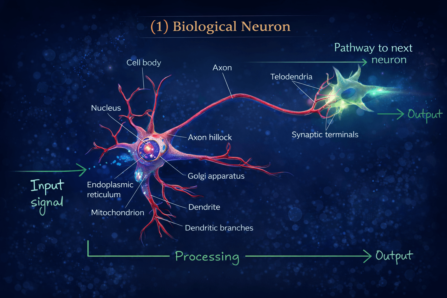
Our brain uses the extremely large interconnected network of neurons for information processing and to model the world around us. Simply put, a neuron collects inputs from other neurons using dendrites. The neuron sums all the inputs and if the resulting value is greater than a threshold, it fires. The fired signal is then sent to other connected neurons through the axon.

Artificial Neuron

Artificial neurons (also called Perceptrons, Units, or Nodes) are the simplest elements or building blocks in an artificial neural network. They are inspired by biological neurons that are found in the human brain.

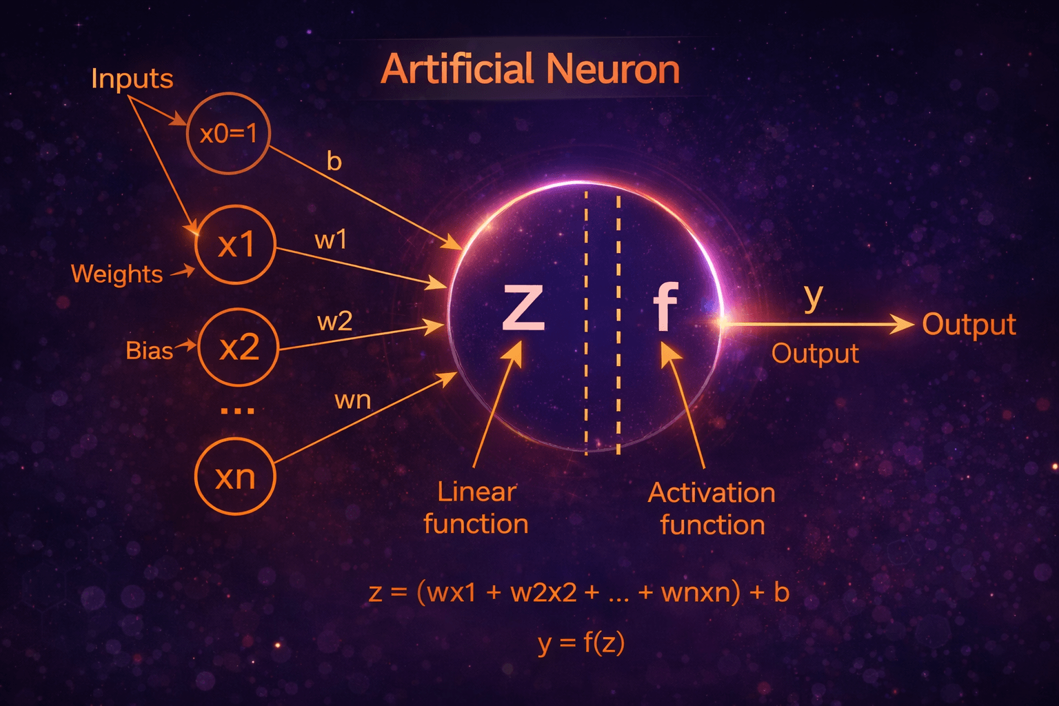
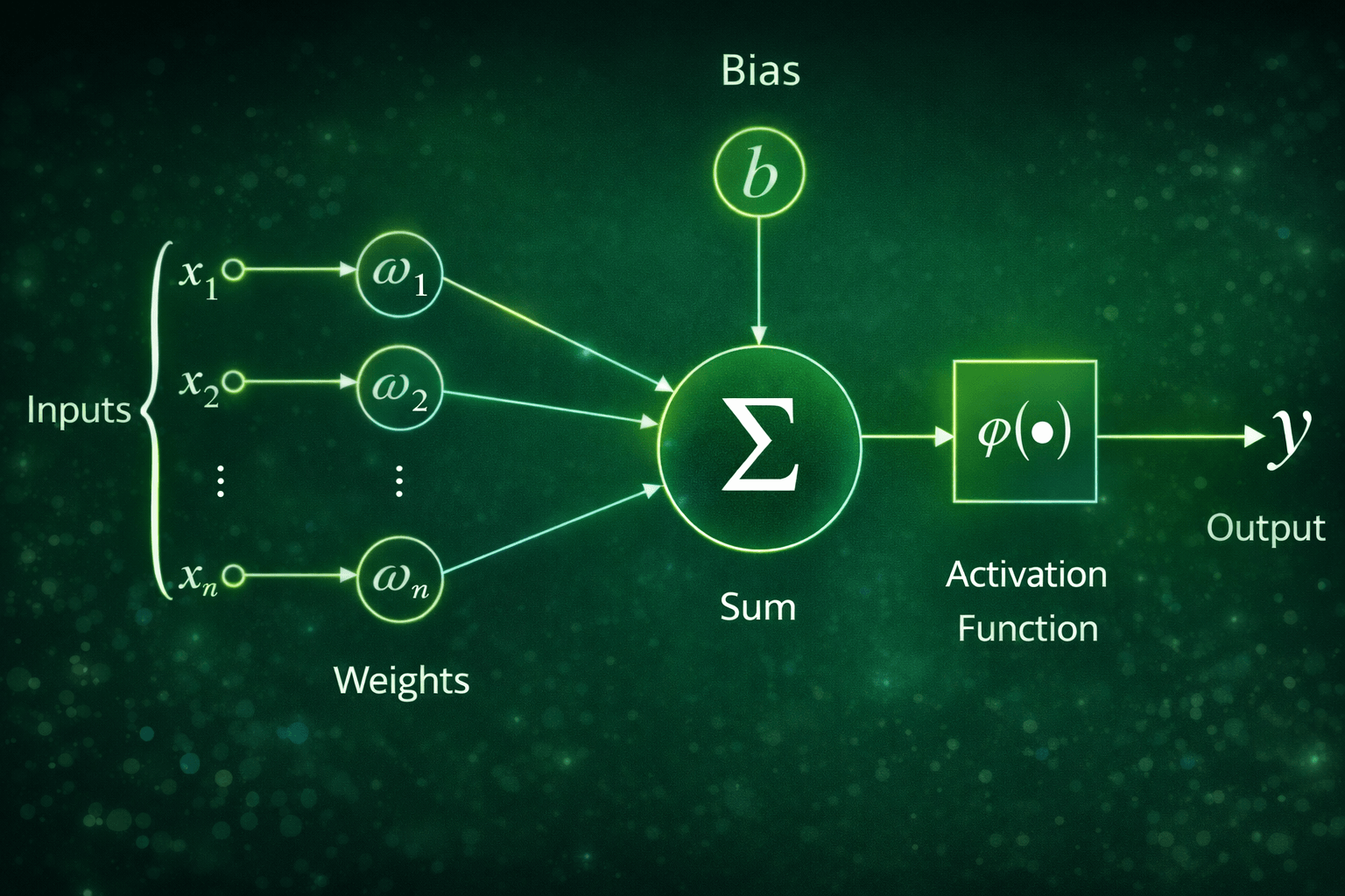
A perceptron takes the inputs, x1, x2, …, xn, multiplies them by weights, w1, w2, …, wn, and adds the bias term, b, then computes the linear function, z on which an activation function, f is applied to get the output, y.

The weights and biases are called the parameters in a neural network model. The optimal values for those parameters are found during the neural network's learning (training) process.

The Z is the linear function, which is the summation of 

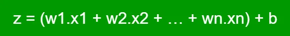
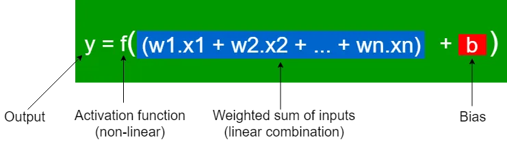
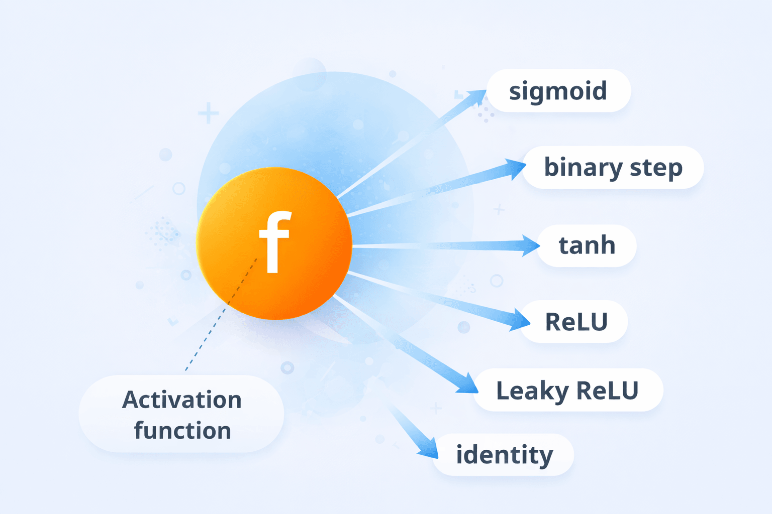
The f is the Activation function, this is also called the non-linear component of the perceptron. It is denoted by f. It is applied on z to get the output y based on the type of activation function we use.

The activation function can be of different types:

How do neural networks work?

Every neural network model consists of layers of nodes, or artificial neurons—an input layer, one or more hidden layers, and an output layer. Each node connects to others, and has its own associated weight and threshold. If the output of any individual node is above the specified threshold value, that node is activated, sending data to the next layer of the network. Otherwise, no data is passed along to the next layer of the network.

Simple neural network model architecture

A basic neural network model has interconnected artificial neurons in three layers:

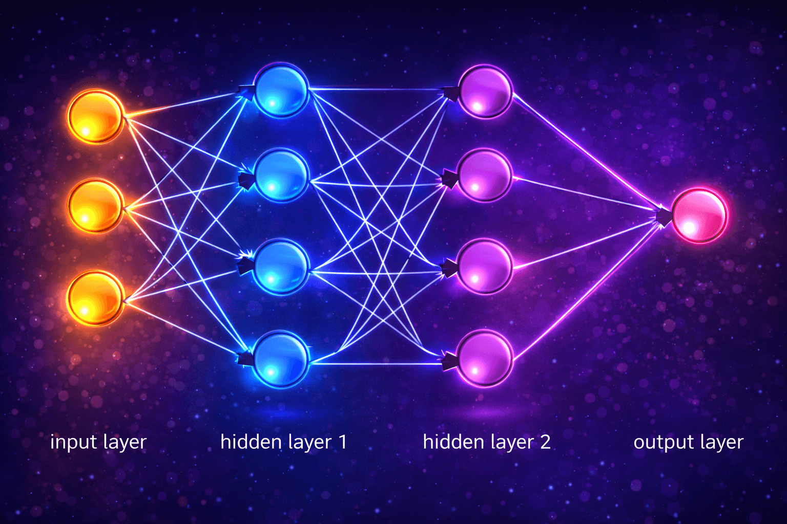
Layers in Neural Network

Input Layer

Information from the outside world enters the artificial neural network from the input layer. Input nodes process the data, analyze or categorize it, and pass it on to the next layer.

Hidden Layer

Hidden layers take their input from the input layer or other hidden layers. Artificial neural networks can have a large number of hidden layers. Each hidden layer analyzes the output from the previous layer, processes it further, and passes it on to the next layer. The hidden layer(s) are where the black magic happens in neural networks. Each layer is trying to learn different aspects of the data by minimizing an error/cost function. The most intuitive way to understand these layers is in the context of 'image recognition' such as a face. The first layer may learn edge detection, the second may detect eyes, the third a nose, etc. This is not exactly what is happening but the idea is to break the problem up into components that different levels of abstraction can piece together much like our own brains work (hence the name 'neural networks').

Output Layer

The output layer gives the final result of all the data processing by the artificial neural network. It can have single or multiple nodes. For instance, if we have a binary (yes/no) classification problem, the output layer will have one output node, which will give the result as 1 or 0. However, if we have a multi-class classification problem, the output layer might consist of more than one output node.

Types of Neural Networks

Artificial Neural networks can be categorized by how the data flows from the input node to the output node.
Multiple types of artificial neural networks are used for advanced machine-learning applications. We don’t have one model architecture that works for all. Neural networks can be classified into different types, which are used for different purposes.

Feedforward Neural Network

A feedforward neural network is one of the simplest types of artificial neural networks devised. In this network, the information moves in only one direction—forward—from the input nodes, through the hidden nodes (if any), and to the output nodes. There are no cycles or loops in the network. Feedforward neural networks were the first type of artificial neural network invented and are simpler than their counterparts.

Architecture of Feedforward Neural Networks

The architecture of a feedforward neural network consists of three types of layers: the input layer, hidden layers, and the output layer as mentioned above. Each layer is made up of units known as neurons, and the layers are interconnected by weights.

How Feedforward Neural Networks Work

The working of a feedforward neural network involves two phases: the feedforward phase and the backpropogation phase.

Feedforward Phase: In this phase, the input data is fed into the network, and it propagates forward through the network. At each hidden layer, the weighted sum of the inputs is calculated and passed through an activation function, which introduces non-linearity into the model. This process continues until the output layer is reached, and a prediction is made.
Backpropagation Phase: Once a prediction is made, the error (difference between the predicted output and the actual output) is calculated. This error is then propagated back through the network, and the weights are adjusted to minimize this error. The process of adjusting weights is typically done using a gradient descent optimization algorithm.
Cost Function in Feedforward Neural Network
‍The cost function is an important factor of a feedforward neural network. Generally, minor adjustments to weights and biases have little effect on the categorized data points. Thus, a method for improving performance can be determined by making minor adjustments to weights and biases using a smooth cost function.

The mean square error cost function is defined as follows:

 Where,
w = weights collected in the network
b = biases
a = output vectors
x = input
‖v‖ = usual length of vector v

Loss Function in Feedforward Neural Network

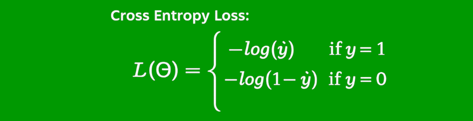
The cross-entropy loss associated with multi-class categorization is as follows:

Applications of Feedforward Neural Networks

Feedforward neural networks are used in a variety of machine learning tasks including:

• Data Compression.
• Pattern Recognition.
• Computer Vision.
• Sonar Target Recognition.
• Speech Recognition.
• Handwritten Characters Recognition

Despite their simplicity, feedforward neural networks can model complex relationships in data and have been the foundation for more complex neural network architectures.

Challenges and Limitations

While feedforward neural networks are powerful, they come with their own set of challenges and limitations. 

1. One of the main challenges is the choice of the number of hidden layers and the number of neurons in each layer, which can significantly affect the performance of the network.
2. Overfitting is another common issue where the network learns the training data too well, including the noise, and performs poorly on new, unseen data.

In conclusion, feedforward neural networks are a foundational concept in the field of neural networks and deep learning. They provide a straightforward approach to modeling data and making predictions and have paved the way for more advanced neural network architectures used in modern artificial intelligence applications.

Convolutional Neural Network(CNN)

A convolutional neural network (CNN) is a category of machine learning model, namely a type of deep learning algorithm well suited to analyzing visual data. CNNs -- sometimes referred to as convnets -- use principles from linear algebra, particularly convolution operations, to extract features and identify patterns within images. Although CNNs are predominantly used to process images, they can also be adapted to work with audio and other signal data.

CNN architecture

The key characteristics of CNNs are:

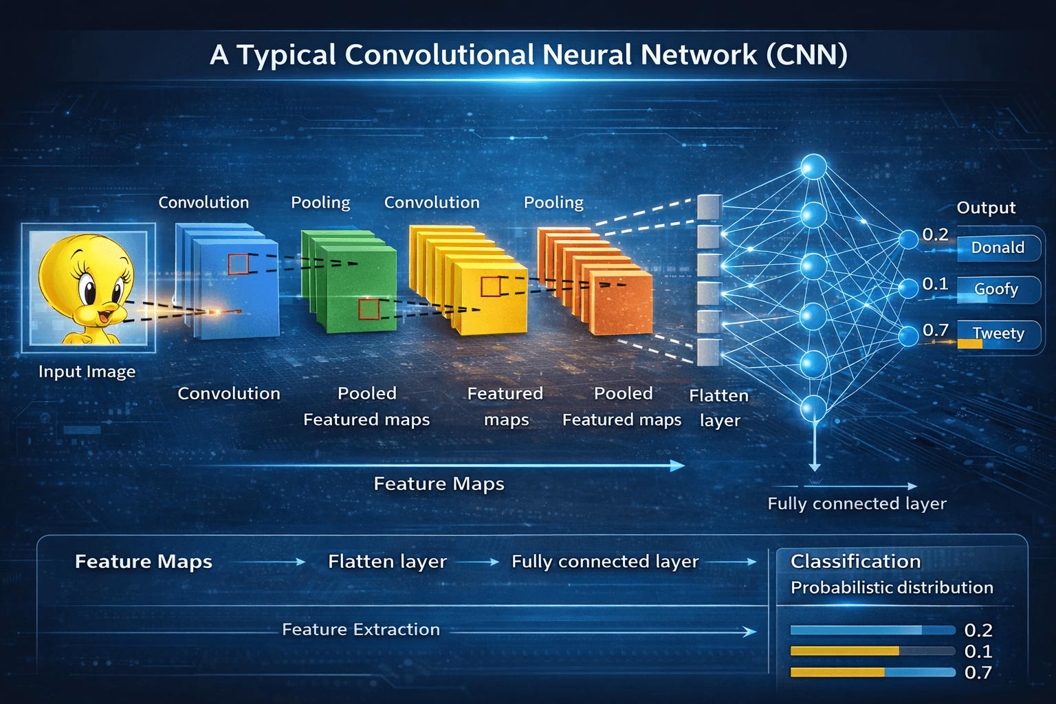
Convolutional layers: These layers use small squares of weights (kernels) to scan the input data, performing a dot product at each location to generate a feature map. This process is known as a convolution operation.
Pooling layers: After convolutional layers, pooling layers are used to reduce the spatial dimensions of the feature maps, reducing the number of parameters and the number of computations required.
Flattening: The output of the pooling layers is flattened into a one-dimensional representation, which is then fed into fully connected layers.
Fully connected layers: These layers are similar to those used in traditional neural networks but with a larger number of neurons and a smaller number of inputs.

CNN architecture is inspired by the connectivity patterns of the human brain -- in particular, the visual cortex, which plays an essential role in perceiving and processing visual stimuli. The artificial neurons in a CNN are arranged to efficiently interpret visual information, enabling these models to process entire images.
CNNs use a series of layers, each of which detects different features of an input image. Depending on the complexity of its intended purpose, a convolutional neural network can contain dozens, hundreds, or even thousands of layers, each building on the outputs of previous layers to recognize detailed patterns.

The process starts by sliding a filter designed to detect certain features over the input image, a process known as the convolution operation (hence the name "convolutional neural network"). The result of this process is a feature map that highlights the presence of the detected features in the image. This feature map then serves as input for the next layer, enabling a convolutional neural network to gradually build a hierarchical representation of the image.

Initial filters usually detect basic features, such as lines or simple textures. Subsequent layers' filters are more complex, combining the basic features identified earlier to recognize more complex patterns. For example, after an initial layer detects the presence of edges, a deeper layer could use that information to start identifying shapes.
Between these layers, the network takes steps to reduce the spatial dimensions of the feature maps to improve efficiency and accuracy. In the final layers of a convolutional neural network, the model makes a final decision -- for example, classifying an object in an image -- based on the output from the previous layers.

A convolutional neural network typically consists of several layers, which can be broadly categorized into three groups: convolutional layers, pooling layers and fully connected layers. As data passes through these layers, the complexity of the CNN increases, which lets the CNN successively identify larger portions of an image and more abstract features.

The benefits of CNNs:

Translation equivariance: CNNs are invariant to translations of the input data, which makes them well-suited for image processing tasks.

Robustness to small distortions: CNNs can learn to recognize patterns despite small distortions or noise in the input data.

Reduced number of parameters: CNNs have fewer parameters than fully connected networks, making them more efficient to train and deploy.

Applications of CNNs:

Image classification: CNNs are widely used for image classification tasks, such as recognizing objects in images or detecting anomalies.
Object detection: CNNs can be used for object detection tasks, such as detecting pedestrians or vehicles in images or videos. CNN's ability to learn visual data has made it a commonly used tool for deep learning in video games.
Image segmentation: CNNs can be used for image segmentation tasks, such as segmenting objects from the background or detecting specific features in an image.
Natural language processing: CNNs can be used for natural language processing tasks, such as text classification or language modeling.
Healthcare: In the healthcare sector, CNNs are used to assist in medical diagnostics and imaging. For example, a CNN could analyze medical images such as X-rays or pathology slides to detect anomalies indicative of disease, thereby aiding in diagnosis and treatment planning.

Types of CNN architectures:

LeNet-5: A simple CNN architecture that was one of the first deep learning models to achieve high accuracy on image recognition tasks.
AlexNet: A deep CNN architecture that won the ImageNet Large Scale Visual Recognition Challenge (ILSVRC) in 2012.
VGGNet: A CNN architecture that uses small convolutional filters and achieves high accuracy on image recognition tasks.
ResNet: A residual network architecture that uses skip connections to ease the training process and achieve high accuracy on image recognition tasks.
InceptionNet: A CNN architecture that uses multiple parallel branches with different filter sizes to capture features at multiple scales.

Challenges

Computational Complexity: CNNs require significant computational resources and memory, especially for large-scale datasets(training samples).
Overfitting: CNNs can overfit to small datasets, especially if not regularized properly.
Limited Interpretability: CNNs can be difficult to interpret, especially for complex models with many layers.

Recurrent Neural Network(RNN)

A recurrent neural network (RNN) is a type of artificial neural network that uses sequential data or time series data. Like feedforward and convolutional neural networks (CNNs), recurrent neural networks utilize training data to learn. They are distinguished by their “memory” as they take information from prior inputs to influence the current input and output. While traditional deep neural networks assume that inputs and outputs are independent of each other, the output of recurrent neural networks depends on the prior elements within the sequence. While future events would also help determine the output of a given sequence, unidirectional recurrent neural networks cannot account for these events in their predictions.

Key Components:

Memory cells: RNNs have a feedback loop that allows them to store information from previous time steps. This is achieved through the use of memory cells, which are essentially nodes that maintain a hidden state.
Hidden state: The hidden state is the internal representation of the RNN's memory. It is updated at each time step based on the input and the previous hidden state.
Cell state: The cell state is an additional memory component that is used to store information that is not immediately needed for the current time step.

Types of RNNs:

Simple RNNs: These are the most basic type of RNNs, which update the hidden state at each time step using a simple recurrence formula.
Long Short-Term Memory (LSTM) Networks: LSTMs are a type of RNN that uses memory cells to store information for longer periods of time. They are particularly effective in handling long-term dependencies.
Gated Recurrent Units (GRUs): GRUs are similar to LSTMs but with fewer parameters and less computational requirements.

RNN Architecture

The architecture of a basic recurrent network consists of the following components:

1. Input Layer: The input layer represents the input features for each time step in the sequence.
2. Recurrent Connection: The key feature of an RNN is the recurrent connection, which allows information to persist across different time steps. At each time step, the hidden state from the previous time step is used in combination with the current input to produce the output and update the hidden state.
3. Hidden State: The hidden state captures information about previous inputs in the sequence. It is updated at each time step based on the current input and the previous hidden state.
4. Output Layer: The output layer produces the output for the current time step based on the current input and the hidden state.

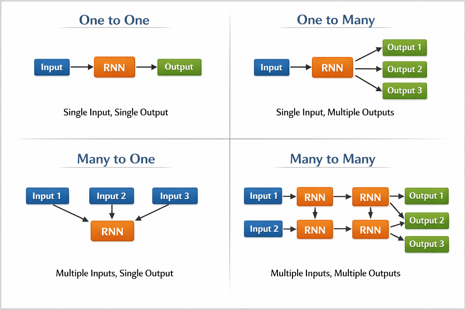
RNN architecture can vary depending on the problem you’re trying to solve. From those with a single input and output to those with many (with variations between).

Below are some examples of RNN architectures that can help you better understand this.

• One To One: There is only one pair here. A one-to-one architecture is used in traditional neural networks.
• One To Many: A single input in a one-to-many network might result in numerous outputs. One too many networks are used in the production of music, for example.
• Many To One:  In this scenario, a single output is produced by combining many inputs from distinct time steps. Sentiment analysis and emotion identification use such networks, in which the class label is determined by a sequence of words.
• Many To Many: For many to many, there are numerous options. Two inputs yield three outputs. Machine translation systems, such as English to French or vice versa translation systems, use many to many networks.

Applications

Language Modeling: Recurrent networks are widely used in natural language processing tasks, such as language modeling, machine translation, and text summarization.
Speech Recognition: RNNs can be used to recognize speech patterns and transcribe spoken language into text.
Time Series Analysis: RNNs can be used to analyze and predict time series data, such as stock prices or weather patterns.

Challenges:

Vanishing Gradients: RNNs can suffer from vanishing gradients, which makes it difficult to train deep networks.
Exploding Gradients: RNNs can also suffer from exploding gradients, which causes the gradients to become too large during training.
Overfitting: RNNs can be prone to overfitting, especially when dealing with small datasets.

Generative Adversarial Networks(GANs)

Generative Adversarial Networks, or GANs for short, is an approach to generative modeling using deep learning methods, such as convolutional neural networks.

Generative modeling is an unsupervised learning task in machine learning that involves automatically discovering and learning the regularities or patterns in input data in such a way that the model can be used to generate or output new examples that plausibly could have been drawn from the original dataset.

How it works

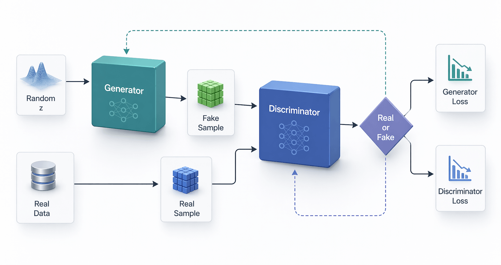
A generative adversarial network system comprises two deep neural networks—the generator network and the discriminator network. Both networks train in an adversarial game, where one tries to generate new data, and the other attempts to predict if the output is fake or real data.

Technically, the GAN works as follows. A complex mathematical equation forms the basis of the entire computing process, but this is a simplistic overview:

1. The generator neural network analyzes the training set and identifies data attributes
2. The discriminator neural network also analyzes the initial training data and distinguishes between the attributes independently
3. The generator modifies some data attributes by adding noise (or random changes) to certain attributes
4. The generator passes the modified data to the discriminator
5. The discriminator calculates the probability that the generated output belongs to the original dataset
6. The discriminator gives some guidance to the generator to reduce the noise vector randomization in the next cycle

The generator attempts to maximize the probability of mistake by the discriminator, but the discriminator attempts to minimize the probability of error. In training iterations, both the generator and discriminator evolve and confront each other continuously until they reach an equilibrium state. In the equilibrium state, the discriminator can no longer recognize synthesized data. At this point, the training process is over.

Key concepts:

Loss functions: The generator's loss/cost function is typically a reconstruction loss (e.g., mean squared error) between the generated sample and the target distribution. The discriminator's loss/cost function is typically a binary cross-entropy loss between its output and the ground truth label (real or fake).
Optimization: Both networks are optimized using backpropagation and stochastic gradient descent.
Mode collapse: A common issue in GANs where the generator produces limited variations of the same output, rather than diverse samples.

Applications

Generating human faces. GANs can produce accurate representations of human faces. For example, StyleGAN2 from Nvidia can produce excellent, photorealistic images of people that don't exist. These pictures are so lifelike that many people believe they're actual individuals.
Developing new fashion designs. GANs can be used to create new fashion designs that reflect existing ones. For instance, clothing retailer H&M used GANs to create new apparel designs for its merchandise.
Creating realistic animal images. GANs can also generate realistic images of animals. For example, BigGAN, a GAN model developed by Google researchers, can produce high-quality images of animals such as birds and dogs.
Video game creation. GANs can be used to create new characters for video games. For example, Nvidia created new characters using GANs for the well-known video game Final Fantasy XV.
Generating realistic three-dimensional (3D) objects. GANs are also capable of producing actual 3D objects. For example, researchers at the Massachusetts Institute of Technology have created 3D models of chairs and other furniture that appear to have been created by people using GANs. These models can be applied to architectural visualization or video games.

Challenges:

Unstable training: GANs can be difficult to train due to the adversarial nature of the process.
Mode collapse: The generator may produce limited variations of the same output. Requires large training samples.
Lack of interpretability: It can be challenging to understand why a particular generator output was produced.

Overall, GANs have shown great promise in generating realistic data and have applications in various fields. However, they require careful tuning and attention to overcome their challenges.

Variational Autoencoders (VAEs)

Variational Autoencoders (VAEs) are a type of deep learning algorithm that uses a probabilistic approach to learn compressed representations of data. They are a type of autoencoder that combines the benefits of generative and variational inference methods.

Basic Idea

A VAE is a neural network that consists of two main components:

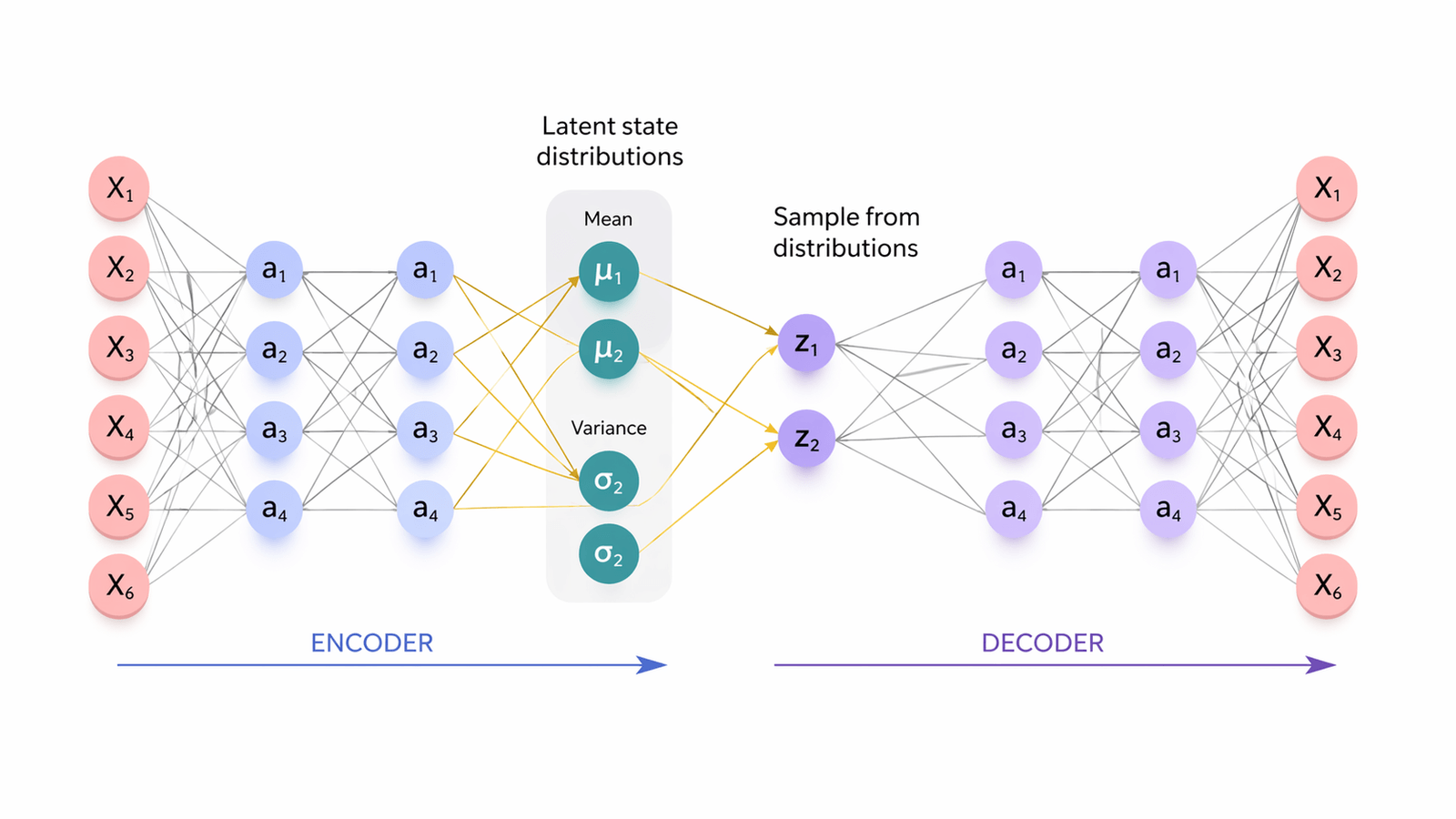
Encoder (or inference network): This network maps the input data to a latent space, where the data is represented by a probability distribution.

Decoder (or generative network): This network maps the latent representation back to the original data space.

The goal of the VAE is to learn a probabilistic mapping between the input data and the latent space, such that the decoded data resembles the original input data. The VAE does this by minimizing the difference between the input data and the decoded data, while also incorporating a regularizer term that encourages the latent representation to be close to a prior distribution.

Key Components

Reparameterization trick: To make it possible to train the VAE using backpropagation, the reparameterization trick is used. This trick involves transforming the random noise in the latent space into a deterministic function of the input data.
Kullback-Leibler (KL) divergence: The KL divergence measures the difference between the posterior distribution and the prior distribution in the latent space. The VAE minimizes this divergence to ensure that the latent representation is close to the prior distribution.
Latent space: The latent space is a lower-dimensional representation of the input data, which is used to capture its underlying structure and patterns.

Architecture of Variational Autoencoder

• The encoder-decoder architecture lies at the heart of Variational Autoencoders (VAEs), distinguishing them from traditional autoencoders. The encoder network takes raw input data and transforms it into a probability distribution within the latent space.
• The latent code generated by the encoder is a probabilistic encoding, allowing the VAE to express not just a single point in the latent space but a distribution of potential representations.
• The decoder network, in turn, takes a sampled point from the latent distribution and reconstructs it back into data space. During training, the model refines both the encoder and decoder parameters to minimize the reconstruction loss – the disparity between the input data and the decoded output. The goal is not just to achieve accurate reconstruction but also to regularize the latent space, ensuring that it conforms to a specified distribution.
• The process involves a delicate balance between two essential components: the reconstruction loss and the regularization term, often represented by the Kullback-Leibler divergence. The reconstruction loss compels the model to accurately reconstruct the input, while the regularization term encourages the latent space to adhere to the chosen distribution, preventing overfitting and promoting generalization.
• By iteratively adjusting these parameters during training, the VAE learns to encode input data into a meaningful latent space representation. This optimized latent code encapsulates the underlying features and structures of the data, facilitating precise reconstruction. The probabilistic nature of the latent space also enables the generation of novel samples by drawing random points from the learned distribution.

Advantages

Interpretable representations: VAEs provide interpretable representations of data by learning a probabilistic mapping between the input data and the latent space.
Flexibility: VAEs can be applied to various types of data, including images, text, and audio.
Robustness: VAEs are robust to outliers and noisy data due to their ability to model uncertainty in the latent space.

Challenges

Training difficulty: Training VAEs can be challenging due to the need to balance reconstruction loss and KL divergence.
Mode collapse: VAEs may suffer from mode collapse, where the generator produces similar outputs for different inputs.
Computational cost: Training VAEs can be computationally expensive due to the need to compute multiple iterations of backpropagation.

Real-world Applications

Generative models for medical imaging: VAEs have been used to generate realistic medical images for diagnosis and treatment planning.
Recommendation systems: VAEs have been used to build recommendation systems that suggest personalized products or services based on user behavior.
Natural language processing: VAEs have been used in natural language processing tasks such as text classification and machine translation.
Drug Discovery and Bioinformatics: In the fields of bioinformatics and drug discovery, VAEs can process and analyze vast amounts of biological data, accelerating the drug discovery process and genetic data interpretation.

The Transformer Model

Transformers are a type of neural network architecture that transforms or changes an input sequence into an output sequence. They do this by learning context and tracking relationships between sequence components. For example, consider this input sequence: "What is the color of the sky?" The transformer model uses an internal mathematical representation that identifies the relevancy and relationship between the words color, sky, and blue. It uses that knowledge to generate the output: "The sky is blue." 

Unlike recurrent neural networks (RNNs) and convolutional neural networks (CNNs), transformers do not use recurrence or convolutional layers. Instead, they use a self-attention mechanism to weigh the importance of different input elements relative to each other.

The paper ‘Attention Is All You Need’ describes transformers

Key Components of a Transformer:

Encoder: The encoder is responsible for transforming input sequences into a continuous representation. It consists of multiple identical layers, each composed of two sub-layers: a self-attention mechanism and a feed-forward neural network (FFNN).
Self-Attention Mechanism: This mechanism allows the model to attend to different parts of the input sequence simultaneously and weigh their importance. It's based on three main components:
Query (Q): The query represents the input sequence.
Key (K): The key represents the input sequence.
Value (V): The value represents the output of the attention mechanism.
Feed-Forward Neural Network (FFNN): This is a fully connected neural network layer with two linear transformations and a ReLU activation function.

How Transformers Work:

Tokenization: The input sequence is broken down into tokens (e.g., words or characters).
Positional Encoding: Each token is assigned a unique positional encoding to preserve the sequence order.
Self-Attention Mechanism: The encoder applies the self-attention mechanism to each token, generating a weighted sum of the input tokens.
Encoder Output: The output of the encoder is a continuous representation of the input sequence.
Decoder: The decoder generates the output sequence one token at a time, using the encoder output and self-attention mechanisms.

The Transformer Architecture

The Transformer architecture follows an encoder-decoder structure but does not rely on recurrence and convolutions to generate an output. 

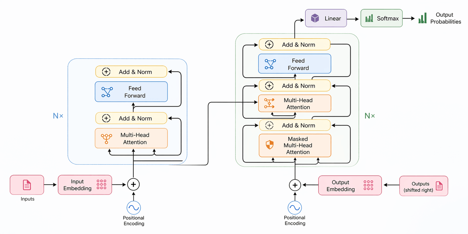
In a nutshell, the task of the encoder, on the left half of the Transformer architecture, is to map an input sequence to a sequence of continuous representations, which is then fed into a decoder. 

The decoder, on the right half of the architecture, receives the output of the encoder together with the decoder output at the previous time step to generate an output sequence.

The Encoder

The encoder consists of a stack of 𝑁= 6 identical layers, where each layer is composed of two sublayers:

1. The first sublayer implements a multi-head self-attention mechanism. The multi-head mechanism implements ℎ heads that receive a (different) linearly projected version of the queries, keys, and values, each to produce ℎoutputs in parallel that are then used to generate a final result. 
2. The second sublayer is a fully connected feed-forward network consisting of two linear transformations with Rectified Linear Unit (ReLU) activation in between:

FFN(𝑥)=ReLU(𝑊1𝑥+𝑏1)𝑊2+𝑏2

The six layers of the Transformer encoder apply the same linear transformations to all the words in the input sequence, but each layer employs different weight (𝑊1,𝑊2) and bias (𝑏1,𝑏2) parameters to do so. 
Furthermore, each of these two sublayers has a residual connection around it.
Each sublayer is also succeeded by a normalization layer, layernorm(.), which normalizes the sum computed between the sublayer input, 𝑥, and the output generated by the sublayer itself, sublayer(𝑥):
layernorm(𝑥+sublayer(𝑥))

An important consideration to keep in mind is that the Transformer architecture cannot inherently capture any information about the relative positions of the words in the sequence since it does not make use of recurrence. This information has to be injected by introducing positional encodings to the input embeddings. 
The positional encoding vectors are of the same dimension as the input embeddings and are generated using sine and cosine functions of different frequencies. Then, they are simply summed to the input embeddings in order to inject the positional information.

The Decoder

The decoder shares several similarities with the encoder. 

The decoder also consists of a stack of 𝑁= 6 identical layers that are each composed of three sublayers:

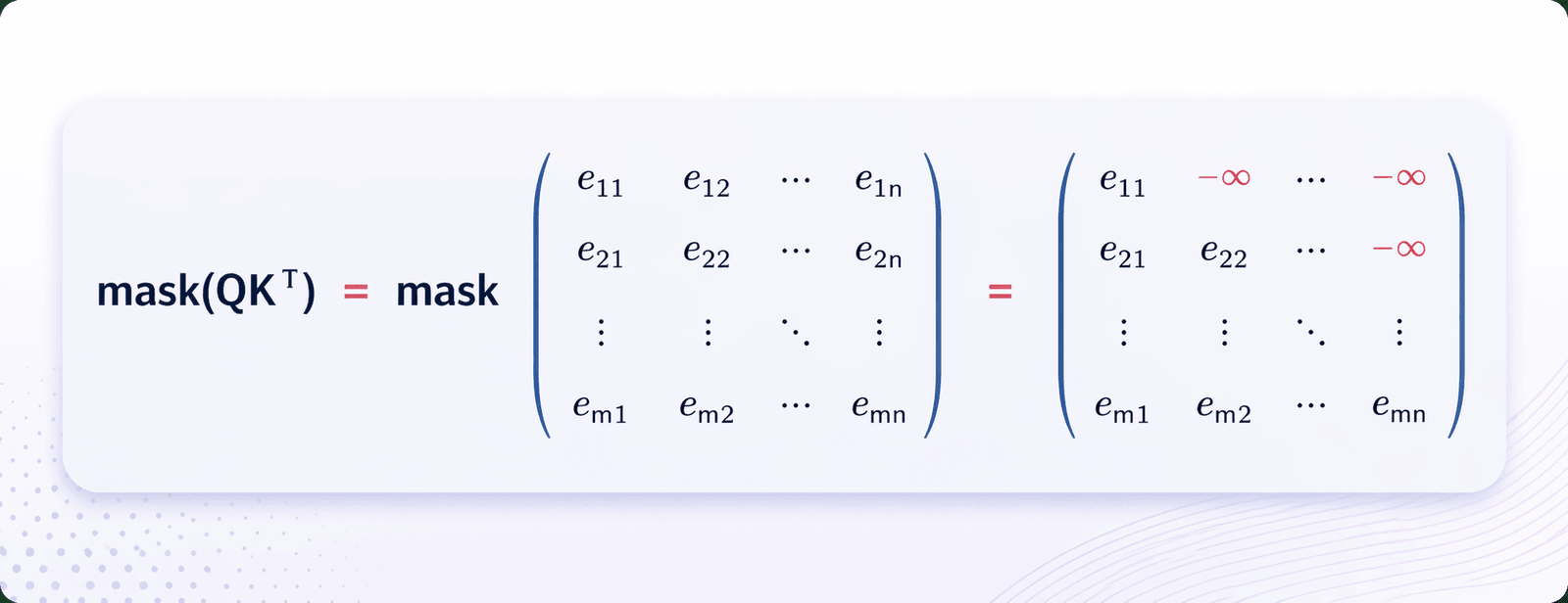
1. The first sublayer receives the previous output of the decoder stack, augments it with positional information, and implements multi-head self-attention over it. While the encoder is designed to attend to all words in the input sequence regardless of their position in the sequence, the decoder is modified to attend only to the preceding words. Hence, the prediction for a word at position 𝑖 can only depend on the known outputs for the words that come before it in the sequence. In the multi-head attention mechanism (which implements multiple, single attention functions in parallel), this is achieved by introducing a mask over the values produced by the scaled multiplication of matrices 𝑄 and 𝐾. This masking is implemented by suppressing the matrix values that would otherwise correspond to illegal connections:

2. The second layer implements a multi-head self-attention mechanism similar to the one implemented in the first sublayer of the encoder. On the decoder side, this multi-head mechanism receives the queries from the previous decoder sublayer and the keys and values from the output of the encoder. This allows the decoder to attend to all the words in the input sequence.
3. The third layer implements a fully connected feed-forward network, similar to the one implemented in the second sublayer of the encoder.

Furthermore, the three sublayers on the decoder side also have residual connections around them and are succeeded by a normalization layer.

Positional encodings are also added to the input embeddings of the decoder in the same manner as previously explained for the encoder. 

Common Transformer Architectures

In the last few years, several architectures based on the basic transformer introduced in the 2017 paper have been developed and trained for complex natural language processing tasks. Some of the most common transformer models that were created recently are listed below:

• BERT
• DistilBERT
• T5
• GPT-2

Applications of Transformers:

Transformers are used in a variety of deep learning/ machine learning tasks

Machine Translation: Transformers have achieved state-of-the-art results in machine translation tasks.
Question Answering: Transformers have been used for question-answering tasks, such as extracting answers from unstructured text.
Text Generation: Transformers have been applied to text generation tasks, such as language modeling and chatbots.
Computer Vision: Transformers have been used in computer vision tasks, such as image generation and object detection.

In summary, transformers are a powerful neural network architecture that has revolutionized the field of NLP and has many applications in various domains. Their ability to process input sequences in parallel and scale to longer inputs has made them an essential tool for many tasks.

‍

Authors

This article is written by Gaurav Sharma, member of 12 of AI, and edited by the 123 of AI team.

‍